Theory

Falling Sphere ViscometerStokes Drag and Terminal Velocity

Fluid MechanicsViscosity

By The Scientist Lounge Team

Introduction

Drop a steel ball bearing into a jar of glycerin and it does not plummet; it glides downward with an almost dignified slowness you can follow with the naked eye. That gentle descent is the everyday signature of viscous drag, and it underlies one of the oldest practical instruments in physics: the falling sphere viscometer. By timing how fast a calibrated bead sinks, an experimenter reads off the thickness of the surrounding fluid.

The motion is so well behaved because a small sphere moving slowly through a thick liquid quickly reaches a balance of forces. Gravity, reduced by buoyancy, pulls it down; a resistive drag pushes back, and once those two match the acceleration vanishes and the speed stops changing. That steady value is the terminal speed, governed for creeping flow by a clean algebraic rule George Stokes derived in 1851.

Here intuition tends to mislead. Faced with two spheres, many people expect the heavier one to plunge dramatically faster, as if weight alone governed the race to the bottom. In the Stokes regime the controlling quantities are radius squared and the density gap between sphere and fluid, while viscosity throttles everything. A denser sphere does settle faster, but only through that density difference, and the relationship is far gentler than raw weight would suggest.

The Physics Explained

A finished run: the sphere has reached the floor and the dimensionless speed curve has flattened onto its dashed terminal-speed asymptote.

Three forces act on the settling sphere. Its weight pulls down with magnitude (4/3)pi r cubed ρ_s g. Buoyancy, the upward push of the displaced fluid, removes (4/3)pi r cubed ρ_f g. The difference is the net driving force, the buoyancy-corrected weight, which depends on the density gap ρ_s minus ρ_f rather than on ρ_s alone. With the default sphere (r = 3 mm, ρ_s = 2500 kg/m3) sinking through glycerin at ρ_f = 1260 kg/m3, that net weight works out to about 0.001376 N.

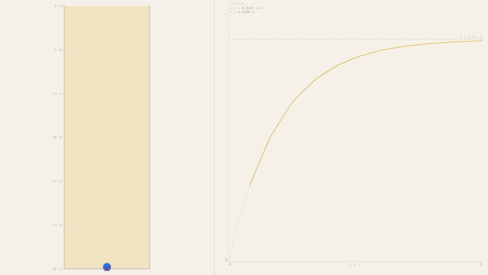
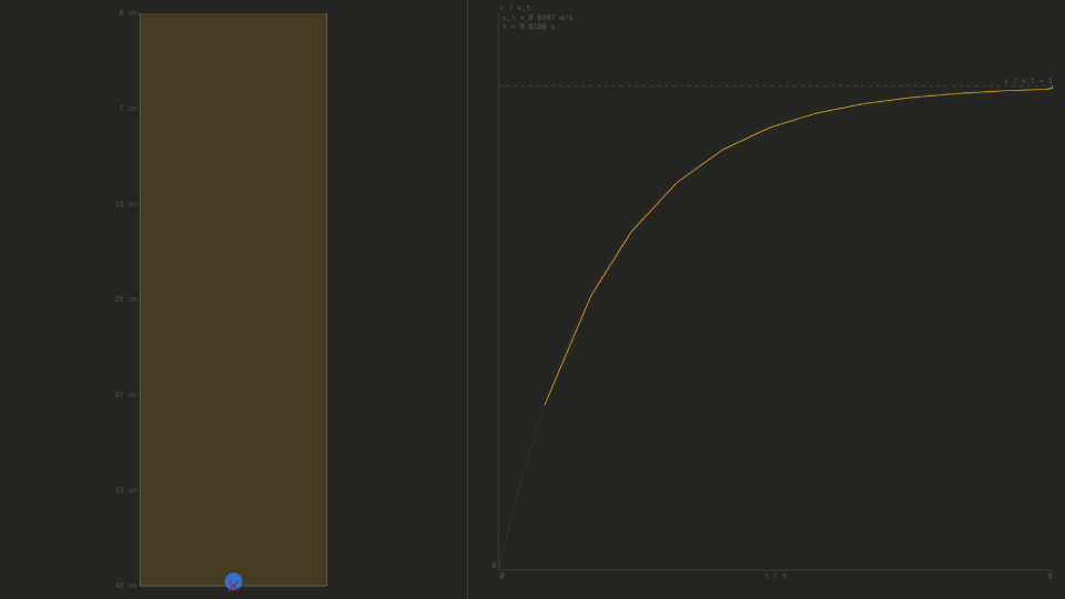
Opposing the descent is Stokes drag, F_d = 6 pi eta r v. The crucial feature is that this resistance grows in direct proportion to speed. At the instant of release the sphere is at rest, so drag is zero and the full net weight accelerates it: the simulator reports an initial downward acceleration near 4.87 m/s2 for the default settings. As the sphere speeds up, drag climbs in step, the net acceleration shrinks, and the speed bends over toward a horizontal asymptote. The right-hand panel plots that approach in dimensionless form, the speed ratio v/v_t against the scaled time t/τ, so every slider setting collapses onto the same universal curve, 1 minus e to the minus t over tau, rising to 1.

The asymptote is the terminal speed, reached when drag exactly cancels the net weight. Setting 6 pi eta r v equal to the buoyancy-corrected weight and solving for v gives the Stokes terminal-velocity formula. At the default configuration the Terminal Speed readout holds at 0.0487 m/s, and the simulated descent speed climbs to and then hugs that value, which on the dimensionless panel is the dashed line at v/v_t = 1. Because drag and net weight balance, the drag force at terminal speed equals the net weight, about 0.001376 N, a force-balance check the simulation honors to numerical precision.

Whether the Stokes picture is trustworthy depends on the Reynolds number, Re = 2 ρ_f r v / eta, which compares fluid inertia to viscous resistance. Stokes drag is exact only when Re is well below one. At the default settings the Reynolds readout sits near 0.74, safely laminar. Lower the viscosity far enough or enlarge the sphere and the rising speed pushes Re past one, at which point an orange warning banner appears: the linear drag law no longer captures the real, partly inertial flow.

Key Equations

Stokes terminal velocity v_t = 2r²(ρ_s − ρ_f)g / (9η)

This is the central result. Inserting the defaults (r = 0.003 m, ρ_s = 2500 kg/m3, ρ_f = 1260 kg/m3, eta = 0.5 Pa.s, g = 9.81 m/s2) gives v_t = 2 times 0.003 squared times 1240 times 9.81 divided by 4.5, which evaluates to 0.218959 / 4.5 = 0.04866 m/s. The Terminal Speed readout rounds this to 0.0487 m/s. Note the radius squared dependence: doubling the radius to 6 mm quadruples the prediction to 0.1946 m/s, while halving eta to 0.25 Pa.s doubles it to 0.0973 m/s.

Stokes drag force F_d = 6πηrv

The drag resisting the descent rises linearly with speed, viscosity, and radius. Evaluated at the default terminal speed (v = 0.04866 m/s, r = 0.003 m, eta = 0.5 Pa.s), it gives 6 times pi times 0.5 times 0.003 times 0.04866, which equals 0.001376 N. That value matches the buoyancy-corrected weight exactly, confirming the force balance that defines terminal speed. Because every factor enters to the first power, the drag at any instant is simply proportional to the current descent speed.

Particle Reynolds number Re = 2ρ_f r v / η

The Reynolds number marks the boundary of validity. Using the default terminal speed (v = 0.04866 m/s, ρ_f = 1260 kg/m3, r = 0.003 m, eta = 0.5 Pa.s) gives 2 times 1260 times 0.003 times 0.04866 divided by 0.5, which is 0.736. Because 0.736 is below one, the flow is laminar and the Stokes formulas hold. When this readout climbs past one, the orange banner flags that the model has left its valid range.

Key Variables

Symbol	Name	Unit	Meaning
r	Sphere radius	m (mm in slider)	Radius of the settling bead; enters terminal speed squared
η	Dynamic viscosity	Pa·s	Thickness of the fluid; the controlling slider, v_t scales as 1/η
ρ_s	Sphere density	kg/m³	Density of the bead material
ρ_f	Fluid density	kg/m³	Density of the glycerin, fixed at 1260 kg/m³
v_t	Terminal speed	m/s	Steady settling speed where drag cancels net weight
Re	Reynolds number	dimensionless	Ratio of inertial to viscous forces; Stokes valid for Re below 1

Real World Examples

How is an unknown fluid's viscosity measured by timing a falling ball?

The falling-sphere viscometer turns settling speed into a measurement. Because terminal speed is inversely proportional to viscosity, a fluid twice as thick lets a calibrated bead settle only half as fast, so reading the speed and rearranging the Stokes formula hands back the unknown viscosity. The simulator pins the relationship down: with r = 3 mm, ρ_s = 2500 kg/m3, and eta = 0.5 Pa.s, the Terminal Speed readout reports 0.0487 m/s. Drag the viscosity slider down to eta = 0.25 Pa.s and that reading climbs to 0.0973 m/s, exactly double, the 1/eta response a real measurement relies on.

This inverse law is the working principle of the falling sphere viscometer itself. An analyst drops a bead of known radius and density into the test liquid, times its descent over a marked length once it has reached steady speed, and rearranges the Stokes formula to solve for the unknown viscosity. Glycerin, honey, motor oils, and molten polymers are all characterized this way, and the method is prized for needing only a stopwatch, a graduated tube, and a calibrated ball.

The catch is that the technique assumes laminar flow. The Reynolds readout reports its validity: at the default settings it holds near 0.74, comfortably inside the creeping-flow band. An experienced analyst checks that number before trusting the result, choosing a bead small and dense enough that the descent stays slow and the inertial terms remain negligible throughout the timed interval.

Where does slow viscous settling matter in nature and industry?

Anyone who has watched a bubble crawl up through a jar of honey, or a spoon sink into cold molasses, has seen this physics directly. In thick syrups and sauces, food scientists care about exactly how fast a suspended particle or air pocket migrates, because it sets a product's shelf life and mouthfeel; the same settling rate decides whether cocoa stays suspended in chocolate or pigment stays even in a tin of paint. Drilling muds are engineered the opposite way, thick enough that rock cuttings settle slowly enough to be carried out of the well.

Biology runs on the same slow descent. Cells, bacteria, and single-celled plankton are dense enough to sink through still water, but only at a creep, which is why a drop of pond water left undisturbed slowly clears as the microorganisms settle out. Laboratories cannot wait for gravity, so a centrifuge multiplies it thousands of times to drive the same Stokes settling in minutes, separating blood into plasma and cells or pelleting a sample by size and density.

At larger scales the principle shapes whole environments. Silt and clay carried by a river drop out where the current slows, building deltas grain by grain as each particle reaches its own settling speed, and water-treatment plants exploit this directly, holding water still in clarifier tanks so suspended solids sink to the bottom and clean water can be drawn off the top. In every case the lesson is the same one the simulator shows: in a viscous fluid, how fast something falls is set by its size, its density, and the thickness of what surrounds it.