Falling Sphere Viscometer · SimulatorStokes Drag and Terminal Velocity
A small dense sphere settles slowly through a viscous liquid (glycerin) in the laminar, low-Reynolds regime where Stokes drag, linear in speed and proportional to viscosity, balances buoyancy-corrected weight. Terminal settling speed scales inversely with viscosity, the controlling slider.
Published: June 20, 2026
Objective
Verify Stokes' Law for a sphere settling through a viscous fluid: terminal speed is inversely proportional to dynamic viscosity and grows as the square of sphere radius. The simulation models the laminar (Re < 1) regime exactly; the Reynolds number readout shows when those idealizations hold.
Setup
- Leave all sliders at defaults (η = 0.5 Pa·s, r = 3 mm, ρ_s = 2500 kg/m³). Note the predicted terminal speed in the vtOut readout before pressing Start.
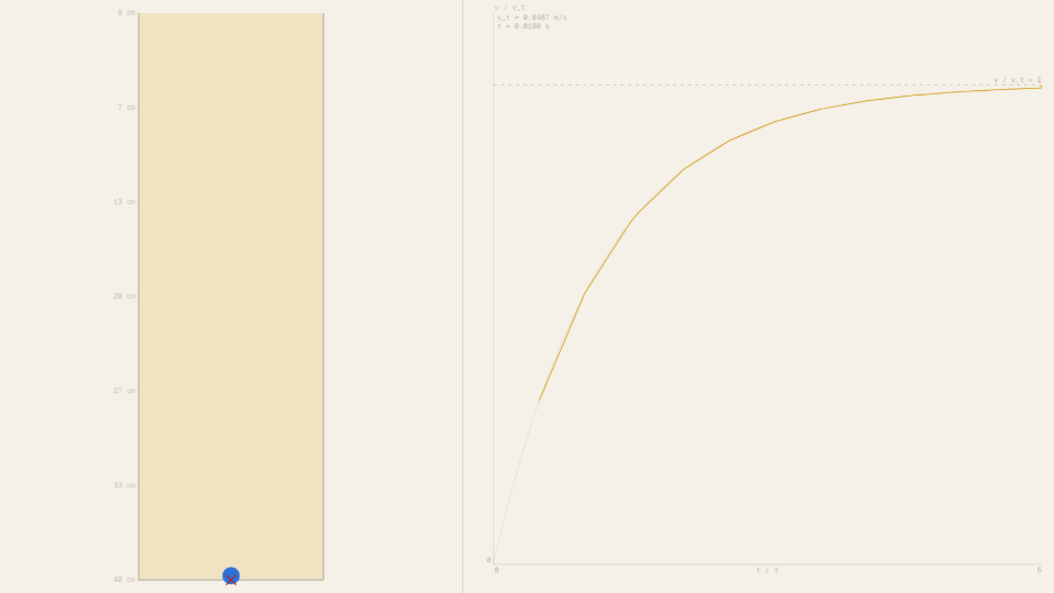
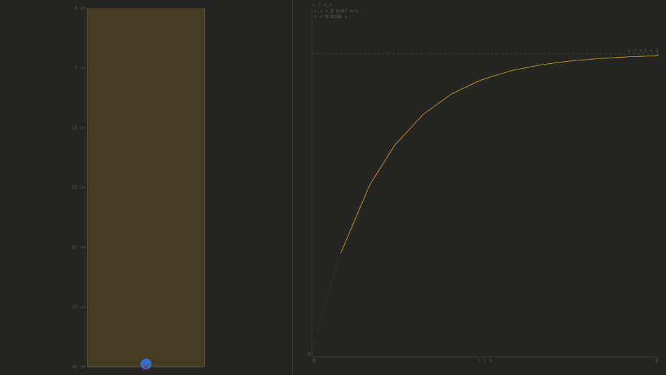
- Press Start and watch the sphere descend. Observe the v(t) graph on the right approaching a plateau. Record the final vOut readout when the sphere reaches the floor.
- Press Reset. Halve the viscosity to η = 0.25 Pa·s and run again. Record the new plateau speed and compare with the first run.
- Reset again. Set viscosity back to 0.5 Pa·s and double the radius to r = 6 mm. Record the terminal speed; compare with the first run to see the r² dependence.
- Reset and set sphere density to ρ_s = 1100 kg/m³ (close to fluid density). Observe the Floats badge when ρ_s falls to 1260 or below.

Analytical Prediction
For a sphere with radius r, density ρ_s, settling through a fluid of density ρ_f = 1260 kg/m³ and viscosity η, Stokes' Law gives terminal speed: v_t = 2r²(ρ_s − ρ_f)g / (9η) With the default config (r = 0.003 m, ρ_s = 2500 kg/m³, η = 0.5 Pa·s):
Halving viscosity to η = 0.25 Pa·s doubles the prediction to ≈ 0.09732 m/s. Doubling radius to r = 6 mm with η = 0.5 Pa·s quadruples it (r² dependence):
The vtOut readout shows the analytic prediction live; vOut tracks the simulation.
Results Analysis
After the sphere reaches the floor, compare vOut (simulation) with vtOut (analytic Stokes formula). The two values should agree within 5 percent for the default configuration. The v(t) graph shows the asymptotic approach to the dashed terminal-speed reference line. When you halve viscosity the plateau doubles, confirming the 1/η scaling. When you double the radius the plateau quadruples, confirming the r² scaling. The Reynolds number readout (reOut) should stay well below 1 in the default configuration (expected Re ≈ 0.74), validating the Stokes model. At low viscosity or large radius, reOut may exceed 1 and the orange warning banner appears, indicating the model is only approximate there.
Source of Error
The simulation models purely laminar Stokes drag (F_d = 6πηrv), which is exact only for Re ≪ 1 and an unbounded fluid. The cylindrical tube creates wall effects that increase the effective drag by a factor of about 1 + 2.1(r/R_tube), neglected here. The sphere is treated as rigid, non-rotating, and the fluid as incompressible and Newtonian. The fluid density is fixed at 1260 kg/m³ (glycerin at roughly 20 °C); temperature dependence of viscosity is omitted. Because both the prediction formula and the simulation share these idealizations, any residual discrepancy between vOut and vtOut is purely numerical rather than physical.
Further Exploration
- Sweep the viscosity slider from its maximum (1.5 Pa·s) down to 0.001 Pa·s. Does the terminal speed change proportionally? At what viscosity does the Reynolds number warning appear, and what does that mean for the Stokes model?
- Set the sphere density just above the fluid density (ρ_s = 1300 kg/m³, η = 0.5 Pa·s). How slowly does the sphere settle? What happens when you reduce density to 1260 kg/m³ or below?
- Compare r = 1 mm versus r = 10 mm at η = 0.5 Pa·s, ρ_s = 2500 kg/m³. Does the ratio of terminal speeds match the predicted factor of (10/1)² = 100?
- Run the default config, then Reset without clearing to accumulate a ghost trace. Change the viscosity and run again. How clearly does the v(t) graph show the inverse relationship between viscosity and terminal speed?