Net Work with Friction PhysicsWork-Energy Theorem & Force Table
Introduction
Net work is the total work done on an object by all forces acting on it, and it equals the object's change in kinetic energy. When a block is pushed across a rough surface, two horizontal forces act simultaneously: the applied push does positive work while kinetic friction does negative work. Adding these contributions gives the net work, which determines exactly how much the block's kinetic energy rises over any displacement.
This accounting matters in every branch of engineering that involves moving parts against resistance. Automotive braking, conveyor belt design, bobsled track analysis, and warehouse floor logistics all reduce to the same question: given a known applied force and a known friction coefficient, how much kinetic energy does the system gain or lose over a given distance? The work-energy theorem, Wnet = ΔKE, answers that question without requiring the full kinematics of the motion.
Most students expect the applied force alone to set the final speed. The simulator's W friction readout contradicts that picture: with F = 25 N, μk = 0.25, m = 3 kg, and d = 10 m, friction removes 73.6 J from the 250 J that the applied force delivers, and the Speed readout settles at 10.84 m/s rather than the 12.91 m/s that ignoring friction would predict.
The Physics Explained
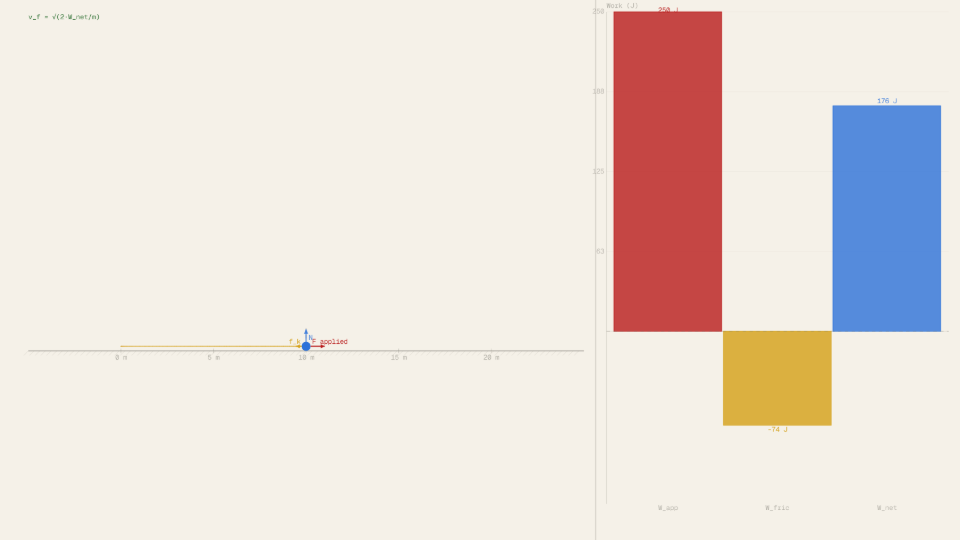
Work is defined as force times displacement in the direction of the force. For the applied force, which acts in the same direction as the block's motion, Wapplied = F · d is always positive. For kinetic friction, which opposes motion, the angle between the friction force and displacement is 180°, so Wfriction = −fk · d is always negative. The simulator computes these continuously as the block moves: the W applied readout tracks F · x in real time, and W friction tracks −μk · m · g · x, where x is the current displacement.
The net work is simply their sum: Wnet = Wapplied + Wfriction = (F − fk) · d. This equals the net force times distance, which is the same as mass times acceleration times distance. Using kinematics, that product equals ½mvf² − ½mvi², confirming the work-energy theorem. With the default configuration of F = 25 N, μk = 0.25, m = 3 kg, d = 10 m, the simulator's W net readout reaches 176.4 J and the KE readout also reads 176.4 J at the track's end, showing both sides of the theorem agree to displayed precision.
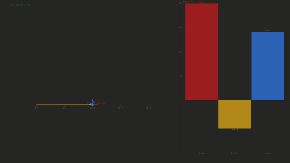
The bar chart on the right half of the canvas visualises the three work quantities simultaneously. The Wapp bar (crimson) grows as positive work; the Wfric bar (amber) grows downward as negative work; the Wnet bar (blue) represents their sum. Watching all three bars update as the block slides across the 10 m track makes the partial and cumulative contributions visible at every instant rather than only at the endpoint.
One boundary case is instructive: when friction exceeds the applied force, the net force is zero or negative and the block never moves. Setting F = 5 N, μk = 0.70, m = 10 kg gives fk = 0.70 × 10 × 9.81 = 68.67 N, which vastly exceeds the 5 N push. The simulator stops immediately with all readouts at zero, illustrating that Wnet = 0 J when Fnet ≤ 0.
Key Equations
With F = 25 N and d = 10 m, this gives Wapplied = 25 × 10 = 250 J. The simulator's W applied readout confirms 250.0 J when the block reaches the end of the track at these settings, matching the equation exactly.
With μk = 0.25, m = 3 kg, g = 9.81 m/s²: fk = 0.25 × 3 × 9.81 = 7.3575 N. This is the constant opposing force the friction arrow on the canvas represents. The work done by this force over d = 10 m is −7.3575 × 10 = −73.575 J, which the W friction readout rounds to −73.6 J.
Continuing the default example: Wnet = (25 − 7.3575) × 10 = 17.6425 × 10 = 176.4 J. The W net readout reports 176.4 J at track end. Both the sum route (250 − 73.6 = 176.4 J) and the net-force route agree, confirming the readout arithmetic.
Setting Wnet = ½mvf² and solving for vf: vf = sqrt(2 · 176.4 / 3) = sqrt(117.6) ≈ 10.84 m/s. The Speed readout displays 10.84 m/s and the KE readout displays 176.4 J at track end, matching both sides of the theorem at the precision shown. The same identity holds for every slider combination where Fnet > 0.
Key Variables
| Symbol | Name | Unit | Meaning |
|---|---|---|---|
| F | Applied force | N | Constant horizontal push on the block, in the direction of motion |
| μk | Kinetic friction coefficient | , | Dimensionless ratio of friction force to normal force for a sliding surface |
| fk | Kinetic friction force | N | Opposing force equal to μk · m · g on a horizontal surface |
| m | Mass | kg | Inertial mass of the sliding block |
| d | Track length / displacement | m | Distance the block travels before the run ends |
| Wnet | Net work | J | Total work by all forces; equals ΔKE by the work-energy theorem |
| vf | Final speed | m/s | Speed at track end, derived from sqrt(2 · Wnet / m) |
| KE | Kinetic energy | J | ½ · m · vf²; equals Wnet when the block starts from rest |
Real World Examples

How does friction determine a car's braking distance?
When a driver applies the brakes, kinetic friction between the tyre and road does negative work on the car, draining its kinetic energy. The work-energy theorem states that Wnet = ΔKE, so the magnitude of the friction work equals the initial kinetic energy that must be removed. With the car treated as a block of mass m moving at speed v, the stopping distance d satisfies μk · m · g · d = ½mv², giving d = v² / (2μk · g).
Doubling the speed therefore quadruples the stopping distance, a result that follows purely from the quadratic relationship between KE and v. The simulator illustrates the underlying friction arithmetic directly: the W friction readout grows as −μk · m · g · x with each metre of displacement, and the same formula governs how far a coasting vehicle travels before rest. Tyre engineers target μk values above 0.7 on dry asphalt to keep stopping distances within safe bounds; the formula shows why even a small drop in μk from wet or worn tyres has a large effect on d because μk enters the denominator of the stopping-distance expression directly.
Setting μk = 0.70 on the simulator with m = 10 kg and F = 5 N reproduces the zero-motion edge case: fk = 68.67 N exceeds the push, all readouts stay at 0 J, and the block never moves. That boundary maps directly onto a tyre with very high grip on a surface where the braking force simply overwhelms any residual forward push.
Why do conveyor belt engineers care about the work done by friction?
A package placed on a moving conveyor belt is initially slower than the belt surface, so kinetic friction acts forward on the package, doing positive work and accelerating it up to belt speed. The same friction does negative work on the belt motor, which must supply extra electrical energy to maintain constant belt speed. The net energy balance is governed by Wnet = ΔKE for the package plus the heat generated at the sliding interface, which equals the friction force times the relative sliding distance.
In the simulator, setting F = 25 N, μk = 0.25, m = 3 kg, d = 10 m gives W applied = 250 J, W friction = −73.6 J, and W net = 176.4 J, with the block reaching vf ≈ 10.84 m/s. A conveyor designer runs the same accounting: the motor must supply at least the net kinetic energy gain of every package plus the frictional heat loss, so minimising μk and the slip distance directly cuts operating costs. That is why rollers with low rolling resistance are preferred over flat belts wherever the product geometry permits.
Raising μk to 0.50 with the same F = 25 N, m = 3 kg, d = 10 m puts fk at 14.72 N, reducing W net to (25 − 14.72) × 10 = 102.8 J and vf to sqrt(2 × 102.8 / 3) ≈ 8.28 m/s. The speed loss from higher friction is exactly what the W net readout reports, confirming that friction's energy toll is neither negligible nor fixed.
How do bobsled engineers use net work to predict finish-line speed?
A bobsled run converts gravitational potential energy into kinetic energy while kinetic friction with the ice continuously removes energy. Over any straight segment, the net work equals the forward component of gravity's work minus the friction work: Wnet = (mg sin θ − μk · mg cos θ) · d. Setting that equal to ΔKE gives the finish-line speed without solving differential equations for the curve geometry.
The simulator captures the flat-surface version of this calculation. With F = 25 N representing the net gravitational push along a slope, μk = 0.25, m = 3 kg, d = 10 m, the W net readout reaches 176.4 J and the Speed readout shows 10.84 m/s, matching vf = sqrt(2 × 176.4 / 3) analytically. Bobsled teams measure ice friction coefficients, typically 0.02 to 0.06, and apply the same net-work formula to estimate run times before competition.
Reducing μk from 0.06 to 0.02 while holding F = 25 N, m = 3 kg, d = 10 m changes fk from 1.77 N to 0.59 N, raising W net from 232.3 J to 244.1 J and vf from 12.43 m/s to 12.74 m/s. That 0.31 m/s gain from runner polishing corresponds to a meaningfully shorter split time across a full 1200 m run, which is exactly the marginal optimisation bobsled engineers pursue.
Further Reading
- Friction block: a detailed look at static and kinetic friction forces on a flat surface, including the transition from rest to sliding and the role of the normal force.
- Friction on an incline: extends the flat-surface friction model to angled surfaces, where the normal force and the friction work both depend on the slope angle.
- Work by a variable force: generalises the constant-force work equation to forces that change with position, using the area under a force-displacement graph.
- Kinetic energy vs velocity: isolates the ½mv² relationship and shows why KE grows quadratically with speed, the same scaling that governs braking distance.