Work by a Variable ForceArea Under F(x) Equals Kinetic Energy
Introduction
The work done by a force that changes along the path is the area under its force-versus-position curve, and by the work-energy theorem that area equals the kinetic energy the object gains. Written as an integral, W = ∫F(x) dx. When the force is constant the integral collapses to the familiar W = F·d, but most forces in nature are not constant: springs stiffen, engines surge, bows pull back harder near full draw.
The intuition that fails here is the constant-force shortcut. With the simulator's default bell-shaped curve peaking at 20 N over a 6 m track, the naive product 20 N × 6 m = 120 J overestimates badly. The peak force acts only near the middle of the track; near both ends the force drops toward 1.81 N. The actual area, which the Work done (J) readout accumulates live, reaches approximately 67.6 J at the end of the run, barely more than half the naive estimate.
The simulator lets you reshape the force profile by dragging five control points, then verifies the theorem for whatever curve you draw: the Work done (J) and Kinetic energy (J) readouts converge to the same number at the finish, every time.
The Physics Explained
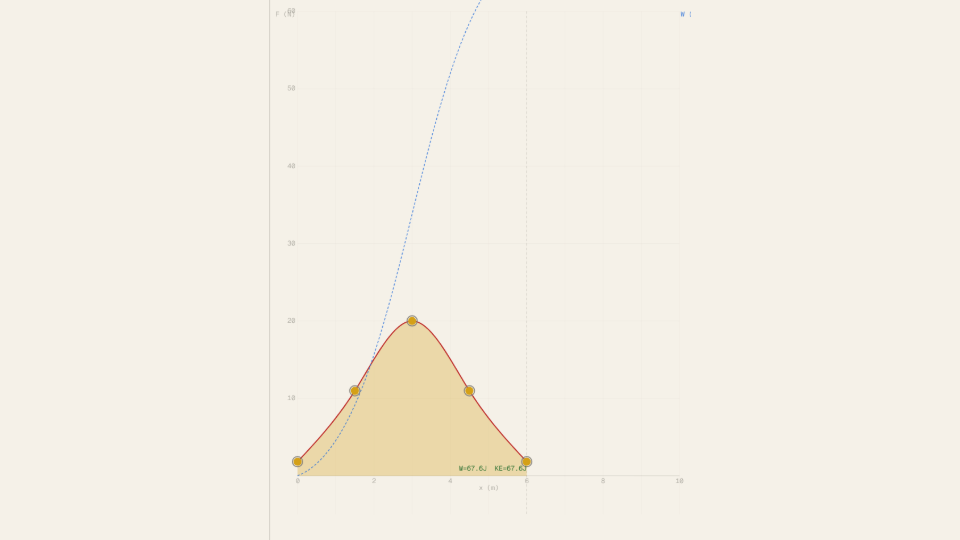
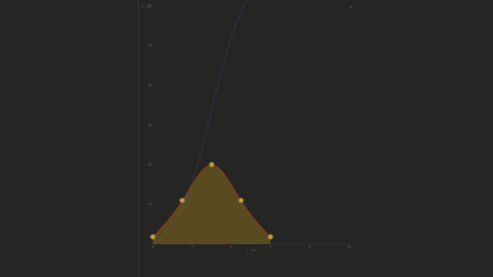
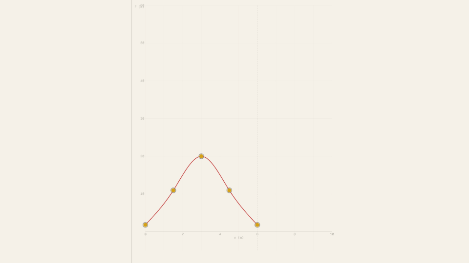
The force profile in the simulator is defined by five draggable control points at fixed positions along the track, joined by a natural cubic spline. At the default settings (mass = 1.0 kg, peak force = 20 N, track length = 6 m) the control points sit at (0, 1.81 N), (1.5, 10.98 N), (3, 20 N), (4.5, 10.98 N), (6, 1.81 N), a symmetric bell. The spline passes smoothly through all five knots and bows slightly above the straight chords between them.
As the block moves, the simulator integrates F(x) numerically with Simpson's rule and shades the accumulated area amber. A rough trapezoid estimate over the four panels between knots gives 9.59 + 23.23 + 23.23 + 9.59 = 65.65 J; the spline's upward bowing adds roughly 2.0 J more, so the true area comes to approximately 67.6 J. That is the number the Work done (J) readout reaches when the block exits the track.
The work-energy theorem closes the loop: every joule of work done by the net force appears as kinetic energy. At the finish, KE = ½mv² must equal W, so the exit speed is v = sqrt(2·W/m) = sqrt(2·67.6/1.0) ≈ 11.6 m/s, which is what the Speed (m/s) readout shows. The sky-blue dashed W(x) overlay traces the running integral and rides along the top edge of the amber shading at every position, a visual statement that the shaded area and the accumulated work are the same quantity.
Because work depends only on the area and not on the shape, very different curves can produce identical outcomes. Doubling every control point by setting the peak force slider to 40 N doubles the area to approximately 135.3 J and raises the exit speed to about 16.4 m/s. Keeping the default curve but halving the mass to 0.5 kg leaves the work unchanged at 67.6 J yet produces that same 16.4 m/s exit speed, because W/m doubles either way. The readouts make this equivalence concrete in a way no formula alone can.
Key Equations
The integral runs from the start of the path to the current position, and geometrically it is the area under the F(x) curve. With the default bell curve the total area over the 6 m track evaluates to approximately 67.6 J. The amber shading in the graph panel is this integral, drawn live as the block advances.
The net work done on an object equals its change in kinetic energy. The block starts from rest (v₀ = 0), so the theorem reduces to W = ½mv², and the exit speed follows as v = sqrt(2·W/m). At the defaults this gives sqrt(2·67.6/1.0) ≈ 11.6 m/s; with the mass slider at 5.0 kg the same work yields sqrt(2·67.6/5.0) ≈ 5.2 m/s.
Sampling the force only at the five control points and joining them with straight lines underestimates the smooth spline. The four 1.5 m panels contribute 9.59 + 23.23 + 23.23 + 9.59 = 65.65 J, about 2.0 J below the spline's 67.6 J, because the cubic segments bow above their chords. Comparing the two estimates is a compact lesson in numerical integration error.
Key Variables
| Symbol | Name | Unit | Meaning |
|---|---|---|---|
| F(x) | Force profile | N | Net force on the block as a function of position, set by five draggable control points |
| x | Position | m | Distance travelled along the track, from 0 to the track length |
| W | Work done | J | Area under F(x) from the start to the current position |
| m | Mass | kg | Mass of the block; ranges from 0.5 to 5.0 kg in the simulator |
| v | Speed | m/s | Instantaneous speed of the block; at the finish v = sqrt(2W/m) |
| KE | Kinetic energy | J | ½mv²; matches the work done at every position on a frictionless track |
Real World Examples
How does an archery bow store energy through a variable draw force?
Drawing a bow is a textbook variable-force process: the force starts near zero at rest and climbs as the string moves back, tracing a draw-force curve that archers measure point by point. The energy stored in the bow is the area under that curve, not the peak force times the draw length.
A compound bow that peaks at 250 N over a 0.6 m draw stores roughly 80 J, noticeably less than the 150 J the naive product suggests, because the force only reaches its peak over part of the draw. When the string is released, that stored area becomes the arrow's kinetic energy: a 0.03 kg arrow leaves at about v = sqrt(2·80/0.03) ≈ 73 m/s.
The simulator makes the same accounting visible. Drag the control points into a bow-like profile, press Start, and the Work done (J) readout accumulates exactly the shaded area that the block converts into speed by the end of the track.
Why does compressing a spring twice as far store four times the energy?
A spring's force grows linearly with compression, F = kx, so the force-position graph is a straight ramp and the stored energy is the area of a triangle: E = ½kx². Doubling the compression doubles both the base and the height of that triangle, quadrupling its area.
A 200 N/m spring compressed 0.10 m holds ½·200·0.10² = 1.0 J; compressed 0.20 m it holds 4.0 J. This is the simplest variable force there is, and it already breaks the constant-force intuition that energy should scale linearly with distance.
In the simulator you can approximate a ramp by dragging the control points to increase steadily from left to right, then watch the Work done (J) readout grow faster and faster as the block advances into the high-force region, exactly as the triangle area predicts.
How do aircraft-carrier catapults shape their force profile to launch jets safely?
A carrier catapult must give a jet a fixed amount of kinetic energy in a track of about 90 m, but it cannot deliver that energy as one violent constant push, because the airframe and the pilot have acceleration limits. Engineers therefore shape the force profile: a controlled rise, a sustained plateau, and a taper near release.
The total area under the curve, and only the area, fixes the exit speed through W = ½mv². Modern electromagnetic launch systems exist precisely because electromagnets can sculpt F(x) far more precisely than steam pistons.
The simulator's draggable control points are a miniature version of that design problem: a sharply peaked curve and a broad flat one can enclose the same area and produce the same exit speed shown in the Speed (m/s) readout, but they load the block very differently along the way, which you can see in how abruptly the Kinetic energy (J) readout climbs.
Further Reading
- Kinetic energy vs velocity: a closer look at the ½mv² relationship that converts the work computed here into the exit speeds the readouts display.
- Pendulum energy bars: energy bookkeeping in a different geometry, where potential and kinetic energy trade places continuously instead of accumulating one way.
- Spring-mass oscillator: the classic linear variable force F = kx, whose triangular force-position area is the ½kx² spring energy discussed in the examples above.