Friction on an Incline PhysicsCritical Angle tan θ = μs
Introduction
Friction on an Incline describes what happens when a block rests on a tilted surface: two friction forces compete with the component of gravity pulling the block downhill. Static friction holds the block in place up to a maximum value set by the surface properties; beyond that limit the block begins to slide, and kinetic friction, always smaller, governs the resulting acceleration. The simulator captures all three forces as labelled vector arrows (weight in crimson, normal in sky blue, friction in amber) and tracks velocity on a live graph, so each regime is directly observable.
The topic appears in every introductory physics course because it ties Newton's second law to a concrete, adjustable geometry. Engineers use the same relationships to design conveyor belts, parking structures, ski-slope grades, and retaining walls. Geotechnical models of landslide risk reduce to the same slip condition. Understanding the critical angle, the tilt at which the block just begins to move, is therefore a gateway to a wide range of applied problems.
Heavier blocks, the reasoning usually goes, should slide at a shallower angle because gravity pulls them harder. The status label says no: with θ = 30°, μs = 0.50, and mass set to any value, the slip condition tan θ = μs is unchanged. Mass cancels out of both sides of the force balance, so the critical angle θc = arctan(μs) ≈ 26.6° is independent of how heavy the block is.
The Physics Explained
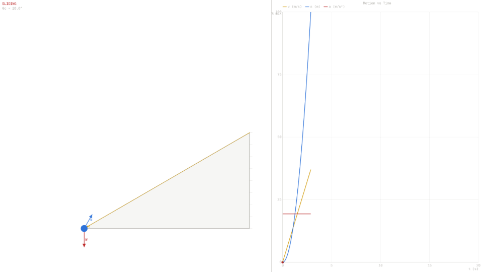
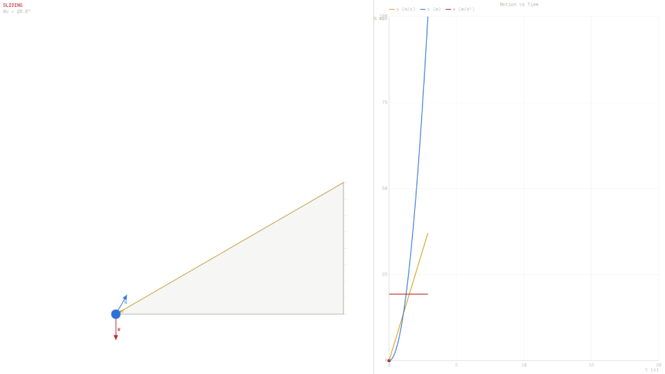
When a block sits on a frictionless incline tilted at angle θ, gravity mg acts straight down. Resolving that force along two axes aligned with the surface reveals the two relevant components: mg·sin θ pulls the block down the slope, and mg·cos θ presses it into the surface. The surface responds with a normal force N = mg·cos θ directed perpendicular to the incline. Static friction acts up the slope and can take any value from zero up to μs·N = μs·mg·cos θ. The block remains stationary as long as mg·sin θ ≤ μs·mg·cos θ, which simplifies to tan θ ≤ μs. The simulator's θc readout displays arctan(μs) continuously, so the gap between the current angle and the slip threshold is always visible.
At the default slider settings (θ = 30°, μs = 0.50, μk = 0.35), the simulator immediately reports SLIDING because tan 30° ≈ 0.577 exceeds μs = 0.50. Once sliding begins, kinetic friction replaces static friction. Its magnitude is fk = μk·mg·cos θ = 0.35·mg·cos 30°, which is smaller than the maximum static value. Applying Newton's second law along the incline gives a net force of mg·sin θ − fk = mg·(sin 30° − 0.35·cos 30°). Dividing by mass yields the acceleration a = g·(sin θ − μk·cos θ). With g = 9.81 m/s², this evaluates to 9.81·(0.500 − 0.303) ≈ 1.93 m/s², matching the Accel. readout the moment the simulation starts.
Switching to a static configuration (θ = 20°, μs = 0.50) demonstrates the other regime. Here tan 20° ≈ 0.364 is well below μs = 0.50, so the friction force only needs to supply 0.364·mg·cos 20° to balance gravity along the slope. Static friction self-adjusts to exactly that value; the block does not move and the acceleration readout holds at 0.00 m/s². The sim pauses automatically after three seconds of continuous static state, confirming that no motion is occurring. The amber friction arrow in the canvas shrinks or grows with the current static demand, making this self-adjustment visible without any additional controls.
The kinetic friction coefficient μk cannot exceed μs; the simulator caps μk at μs (the μk slider's maximum tracks μs) so that the physical ordering μk ≤ μs is never violated regardless of slider positions. This constraint reflects the real observation that once sliding begins, less force is needed to keep the block moving than to start it moving; the Velocity vs Time graph shows the block accelerating smoothly once the static regime ends, with no deceleration back to rest unless the angle is reduced below θc mid-run.
Key Equations
The surface must push back perpendicular to itself with exactly enough force to prevent the block from sinking through. At the default settings of m = 2.0 kg, θ = 30°, g = 9.81 m/s²: N = 2.0·9.81·cos 30° = 2.0·9.81·0.866 = 16.99 N. This is the force that scales both the static friction limit and the kinetic friction magnitude.
Mass cancels from both sides of mg·sin θ = μs·mg·cos θ, leaving the dimensionless ratio tan θ = μs as the threshold. With μs = 0.50, the critical angle is θc = arctan(0.50) ≈ 26.6°. The simulator's θc readout confirms this: at θ = 26° the block stays STATIC; at θ = 27° the status flips to SLIDING, consistent with the arctan formula to within the 1° slider resolution.
Once sliding has begun, friction locks to this fixed value regardless of speed. At the default settings: fk = 0.35·2.0·9.81·cos 30° = 0.35·16.99 = 5.95 N. This acts up the incline, opposing the downhill motion.
Dividing the net force along the incline by mass yields this result, from which mass has again cancelled. At θ = 30°, μk = 0.35: a = 9.81·(sin 30° − 0.35·cos 30°) = 9.81·(0.500 − 0.303) = 9.81·0.197 ≈ 1.93 m/s². The Accel. readout in the simulator displays 1.93 m/s² at t = 0, and the Velocity vs Time graph rises linearly from zero at this slope until the block reaches the bottom of the 8 m ramp at approximately t = 2.88 s.
Key Variables
| Symbol | Name | Unit | Meaning |
|---|---|---|---|
| θ | Incline angle | ° | Tilt of the ramp surface measured from horizontal |
| μs | Static friction coefficient | (none) | Ratio of maximum static friction to normal force; sets the critical angle |
| μk | Kinetic friction coefficient | (none) | Ratio of kinetic friction to normal force while the block is sliding; always less than μs |
| N | Normal force | N | Contact force perpendicular to the incline surface; equals mg·cos θ |
| a | Acceleration | m/s² | Net acceleration along the incline once sliding begins; zero in the static regime |
| θc | Critical angle | ° | Smallest angle at which slipping occurs; equals arctan(μs) |
Real World Examples
Why do engineers tilt conveyor belts at specific angles?
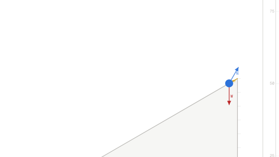
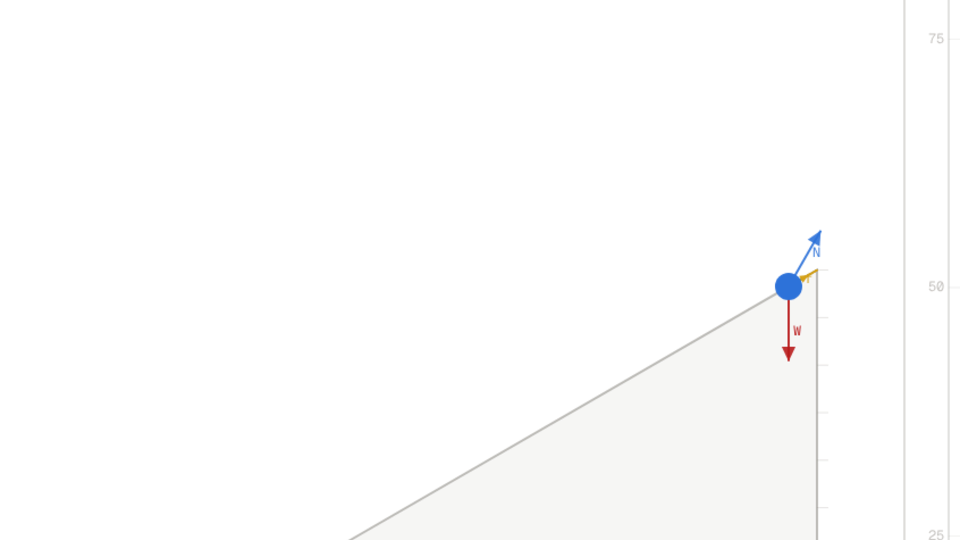
Conveyor belt design requires keeping loose materials stationary relative to the belt surface while the belt moves. If the belt tilts beyond the critical angle θslip = arctan(μs) for the material being carried, particles begin sliding backward, a failure mode that jams the system or spills cargo. Engineers therefore measure the static friction coefficient between the belt material and the cargo, then set the incline angle comfortably below arctan(μs).
For grain on rubber conveyor belting, typical μs values run from 0.55 to 0.70, placing the safe operating ceiling between about 29° and 35°. With μs = 0.50 and θ = 26° in the simulator, the θc readout confirms θc = arctan(0.50) ≈ 26.6°, and the status label holds at STATIC because 26° falls below that threshold. Raising the angle slider to 27° flips the status to SLIDING, demonstrating exactly the margin engineers guard against in real belt designs.
How do automotive engineers set the slope limit for parked cars on hills?
A parked car on a hill relies on static friction between the tire and road surface (supplemented by the parking brake engaging the drivetrain) to resist sliding. The pure friction limit without the brake is governed by tan θ = μs: for a dry asphalt–rubber interface, μs ≈ 0.70, giving a critical angle near 35°. Wet pavement drops μs toward 0.40, pushing θc down to roughly 22°. Municipal parking codes in hilly cities often cap allowable street grades near 17°–20° partly for this reason, keeping a safety margin below the wet-pavement threshold.
The simulator makes the slope sensitivity concrete: with μs = 0.40 and the angle slider at 21°, the block remains STATIC; nudging the angle to 22° triggers SLIDING and the acceleration readout jumps to a = g·(sin 22° − 0.30·cos 22°) ≈ 0.94 m/s² using μk = 0.30, matching the analytical prediction within the displayed precision. The kinetic friction amber arrow visibly shortens compared with the normal sky-blue arrow, reflecting the reduced friction that remains once the block is in motion.
The same analysis applies to loaded trucks, where cargo shifts the effective center of mass but, because mass cancels from the slip condition, does not change the angle at which friction fails. Fleet managers who operate in mountainous terrain therefore specify the road-surface friction rating rather than the vehicle weight class when evaluating slope risk.
How do geologists use the friction angle to predict landslide risk?
Slope stability analysis in geotechnical engineering reduces, in its simplest form, to the same slip condition that governs the simulator: a soil layer slides over bedrock when the hillside angle θ exceeds arctan(μs) for the soil–rock interface. Geologists measure this angle of repose in the laboratory and then map hillside gradients from topographic data. Any slope steeper than θc is classified as conditionally unstable.
A rainstorm that lubricates the interface and drops μs from 0.60 to 0.35 shifts θc from 31° to 19°, potentially destabilising slopes that were previously safe. The simulator illustrates this sensitivity directly: holding the angle slider at 25° and reducing μs from 0.60 to 0.50 keeps the status at STATIC (arctan(0.50) ≈ 26.6°, which remains above 25°); reducing μs further to 0.45 drops θc to 24.2°, which falls below the current angle of 25°, and immediately triggers SLIDING, the same threshold-crossing behaviour that precedes real slope failures.
Once sliding begins, the acceleration a = g·(sin θ − μk·cos θ) determines how quickly the material moves. At θ = 25° and μk = 0.28 (a representative saturated-soil value), the simulator's Accel. readout shows approximately 1.65 m/s², which integrated over tens of seconds produces the velocities observed in slow-moving earthflows. Faster landslides correspond to steeper angles and lower μk values, both of which the angle and coefficient sliders can replicate.
Further Reading
- Inclined plane: the frictionless ramp baseline: how normal force and gravitational components behave before friction is introduced.
- Friction block: static and kinetic friction on a horizontal surface, isolating the coefficient relationship without the angular geometry.
- Free-body diagram builder: construct and inspect the three-force diagram (weight, normal, friction) that underpins the incline analysis.
- Newton's third law carts: how the normal contact force at the surface satisfies the action–reaction pair that the incline problem implicitly relies on.