Two-Rope Tension PhysicsWhy Shallow Angles Spike Tension
Introduction
Two-Rope Tension describes one of the most common configurations in all of statics: a single load hanging from a junction supported by two ropes that rise to fixed anchors. Each rope pulls along its own line, and together with the downward weight the three forces must balance exactly, because nothing is moving. The question the simulator answers is how the load's weight is shared between the two ropes, and how that sharing depends on the angles at which the ropes are strung.
The setup is everywhere once you look for it: a hanging sign, a traffic light strung across an intersection, a picture wire, the slings of a crane lift, a power line, and a tightrope are all two-rope-tension problems. The same force balance decides whether a cable is comfortably loaded or dangerously overstretched, which is why riggers, structural engineers, and arborists all reason about it daily.
Ask anyone how the load divides and the answer comes back half and half, one share per rope. The tension readouts honor that split only in one special case (symmetric ropes at a moderate angle); as the ropes flatten toward horizontal, the tension in each climbs without bound, far exceeding the weight it supports. That counterintuitive amplification is the heart of the topic.
The Physics Explained

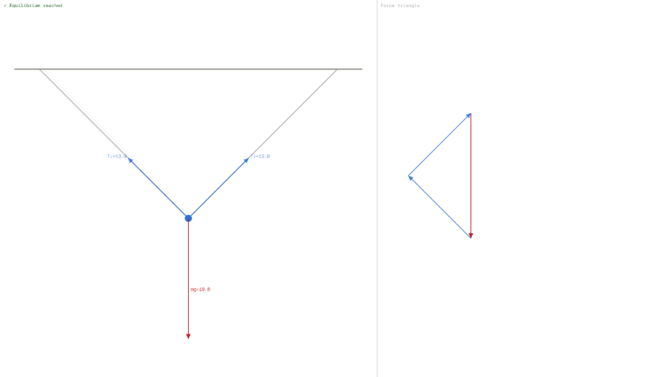
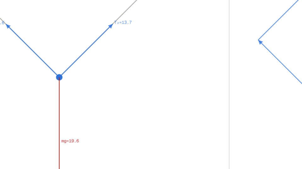
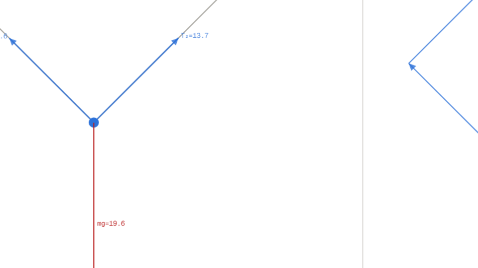
The load hangs from a junction where the two ropes meet. Three forces act there: the weight m·g straight down, the tension T₁ along the left rope, and the tension T₂ along the right rope. Because the junction is in static equilibrium (it is not accelerating), these three forces add to zero. Resolving them into horizontal and vertical components turns that single vector statement into two scalar equations that can be solved for the two unknown tensions.
Horizontally, the only forces are the two tensions, pulling in opposite directions toward their anchors. For the junction to stay put, their horizontal components must cancel: T₁·cos θ₁ = T₂·cos θ₂, where θ₁ and θ₂ are the angles each rope makes above the horizontal. Vertically, the upward pull from both ropes must support the full weight: T₁·sin θ₁ + T₂·sin θ₂ = m·g. These are the two equilibrium conditions, and the simulator displays them directly as the residual readouts ΣFx and ΣFy, which fall to 0.00 N once the load has settled.
Solving the pair gives a closed form for each tension: T₁ = m·g·cos θ₂ ⁄ sin(θ₁ + θ₂) and the mirror expression for T₂. The crucial feature is the denominator sin(θ₁ + θ₂). When the ropes are steep and the angle sum approaches 90°, the denominator is near 1 and the tensions are modest. As the ropes flatten and the angle sum shrinks toward zero, the denominator collapses and the tensions diverge. With a 2.0 kg load and both ropes at 45°, each tension is 13.87 N: slightly above half the 19.62 N weight, not exactly half, because each rope also has to cancel the other's horizontal pull.
It is tempting to expect the two tension magnitudes to add up to the weight, but they do not. Only the vertical components sum to m·g; the magnitudes are larger because part of each tension is spent pulling sideways against the other rope. This is why the simulator reports equilibrium through the component residuals rather than a single "tension equals weight" check. It is also why, on the simulation, the brief tug you see on starting is only a visualization device. In reality the ropes reach these tensions the instant the load is hung, with no swing at all.
Key Equations
The sideways pull of each rope must cancel the other, or the junction would drift horizontally. When the angles are equal this forces the tensions to be equal; when they differ, the rope at the shallower angle must adjust its tension to match the other's horizontal component.
The upward components of the two tensions together carry the entire weight. At the default settings of m = 2.0 kg and g = 9.81 m/s², the load is m·g = 19.62 N, and with both ropes at 45° the two vertical components 13.87·sin 45° each contribute 9.81 N, summing exactly to the weight.
Combining the two balances isolates each tension. With θ₁ = θ₂ = 45°, sin(θ₁ + θ₂) = sin 90° = 1 and cos 45° = 0.7071, giving T₁ = 2.0·9.81·0.7071 ⁄ 1 = 13.87 N. Flattening both ropes to 15° makes sin(θ₁ + θ₂) = sin 30° = 0.5, and each tension rises to 37.9 N, almost double the weight.
Static equilibrium means both residual force components vanish at once. The simulator drives ΣFx and ΣFy to 0.00 N as the load settles; any non-zero reading during the brief starting tug is the system relaxing toward the analytic solution, not a real oscillation.
Key Variables
| Symbol | Name | Unit | Meaning |
|---|---|---|---|
| θ₁ | Left rope angle | ° | Angle the left rope makes above the horizontal at its anchor |
| θ₂ | Right rope angle | ° | Angle the right rope makes above the horizontal at its anchor |
| T₁ | Left tension | N | Force the left rope exerts along its length |
| T₂ | Right tension | N | Force the right rope exerts along its length |
| m | Load mass | kg | Mass of the hanging load; its weight is m·g |
| ΣFx, ΣFy | Force residuals | N | Net horizontal and vertical force at the junction; both zero at equilibrium |
Real World Examples
Why does a tightrope or slackline carry far more tension than the walker's weight?
A tightrope sags only a few degrees below horizontal under a walker, which means both supporting angles θ₁ and θ₂ are small. Tension is governed by T = m·g·cos θ ⁄ sin(θ₁ + θ₂), and when both angles are small the denominator sin(θ₁ + θ₂) is also small, so the tension balloons far above the load's weight.
The simulator makes this concrete. With a 2.0 kg load and both ropes at 45°, each rope carries 13.87 N against a weight of 19.62 N. Drag both angle sliders down to 15° and each tension climbs to 37.9 N, nearly double the weight per rope, even though the load has not changed. A real slackline rated for a 70 kg walker is tensioned to several kilonewtons precisely so that it sags only slightly; the flatter the line, the harder every anchor and the webbing itself must pull, which is why slackline anchors are engineered with large safety margins.
How do riggers choose the angle between two slings lifting a load?
When a crane lifts a load with two slings meeting at a hook, the angle each sling makes with the horizontal sets how much tension it carries; a wider included angle of shallower slings sharply increases that tension. This is the same geometry the simulator models. Keeping the load at 2.0 kg and setting both ropes to 45° puts 13.87 N in each sling; flattening them toward 15° drives each to 37.9 N, so the slings, shackles, and lifting points all see far more force for an unchanged load.
Rigging charts capture this with a sling-angle factor, and the industry rule of thumb is to keep the angle between each sling and the load steep, typically no shallower than 45° to 60° from horizontal. The asymmetric case is just as instructive: setting the left rope to 30° and the right to 60° gives 9.81 N on the left and 16.99 N on the right, showing that when the two sides are not symmetric the geometry redistributes the load unevenly while the horizontal and vertical force balances still hold.
Why do power lines and long cables sag instead of hanging level?
Stretch a cable between two poles and you might expect it could be pulled perfectly straight. The geometry forbids it. A truly level cable would make both angles θ₁ and θ₂ equal to zero, sending sin(θ₁ + θ₂) to zero and the tension T = m·g·cos θ ⁄ sin(θ₁ + θ₂) to infinity. No real cable can supply infinite tension, so every loaded line must sag at least a little; the sag is what gives the supporting forces a vertical component to carry the weight.
The simulator has the same built-in limit: the angle sliders stop at 10°, because going lower drives the tension toward impractical values. With a 2.0 kg load and both ropes at the 10° minimum, each tension reaches 56.5 N, nearly three times the 19.62 N weight. This is why utility companies specify a deliberate sag for every span of power line, and why a guitar string pulled nearly straight at high tension snaps so readily when over-tightened: the flatter the line, the closer it sits to the runaway region of the tension curve.
Further Reading
- Free-body diagram builder: construct and inspect the force diagram that isolates the weight and the two tensions, the foundation of the two-rope analysis.
- Atwood machine: rope tension in a different equilibrium configuration, where two masses are linked over a pulley.
- Newton's third law carts: how the tension in a rope satisfies the action–reaction pair at the load and the anchor.
- Friction on an incline: another problem solved by resolving forces into components along chosen axes.