Circular Motion Vectors PhysicsWhy Acceleration Points Inward
Introduction
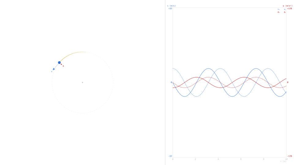
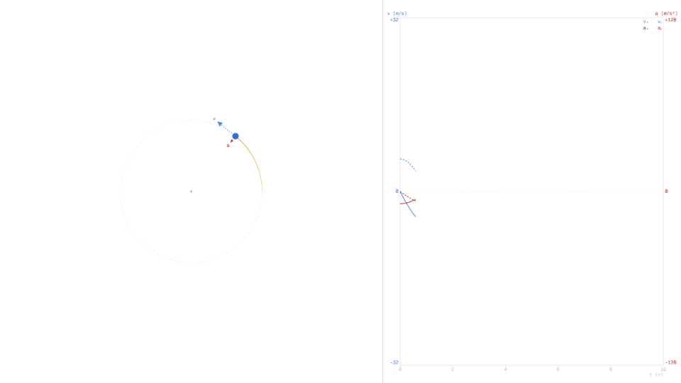
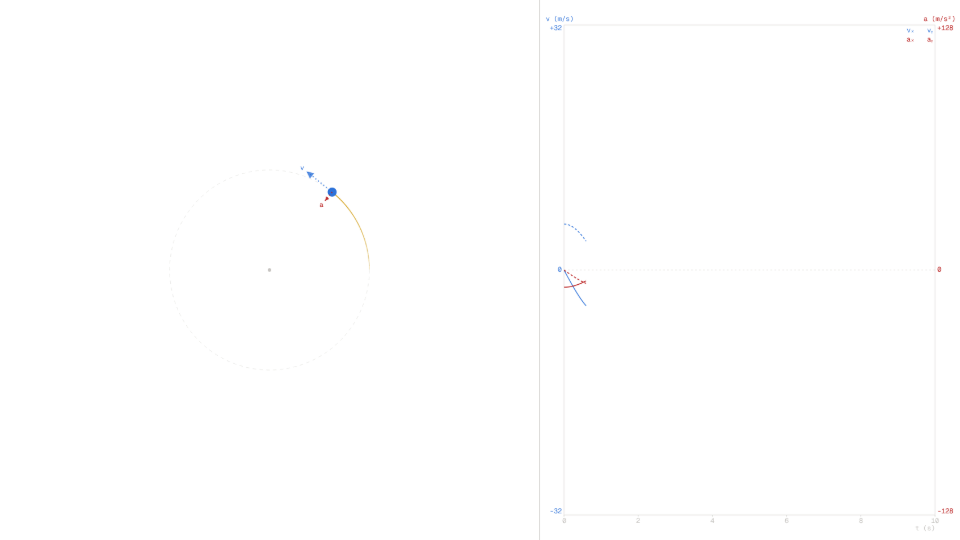
Uniform circular motion occurs when an object travels along a circular path at constant speed. Three vectors describe the state of that object at every instant: a position vector pointing from the centre to the object, a velocity vector tangent to the circle at that point, and a centripetal acceleration vector pointing back toward the centre. All three rotate continuously as the object moves, yet each maintains a fixed relationship to the others: the velocity is always perpendicular to the position vector, and the acceleration is always antiparallel to the position vector.
This corner of kinematics offers the clearest demonstration that acceleration does not require a change in speed, which is why it appears early in every mechanics sequence. A car turning at constant speed, a satellite in low Earth orbit, a centrifuge separating blood plasma: all involve an acceleration that is purely directional. Engineers and physicists routinely decompose more complex curved paths into locally circular arcs, which makes the uniform case the foundational reference for road design, orbital mechanics, and rotating machinery.
It is tempting to conclude that an object moving in a circle at constant speed is not accelerating; after all, the speedometer never changes. The readouts refute that directly: with radius r = 4 m and angular velocity ω = 1.5 rad/s, the centripetal acceleration readout holds steady at 9 m/s² pointing inward while the speed readout stays fixed at 6 m/s. Direction change alone constitutes a real, measurable acceleration.
The Physics Explained
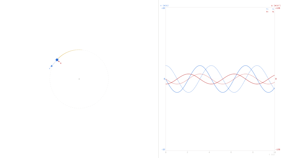
An object undergoing uniform circular motion sweeps through angle θ = ω·t at a constant angular velocity ω. Its position vector has magnitude equal to the radius r and rotates at rate ω. At any instant the position can be resolved into Cartesian components x = r·cos(ω·t) and y = r·sin(ω·t). The simulator draws the position vector from the centre of the track to the object; with r = 4 m and ω = 1 rad/s, that arrow rotates at one radian per second and always has length 4 m regardless of where the object sits on the track.
The velocity vector is the time derivative of the position vector. Differentiating x and y gives vₓ = −r·ω·sin(ω·t) and vy = r·ω·cos(ω·t). The magnitude is v = r·ω, independent of time, confirming constant speed. The direction is perpendicular to the position vector, rotated 90° ahead in the direction of travel. The simulator's velocity arrow always lies tangent to the circle; with r = 4 m and ω = 1.5 rad/s, the speed readout locks at 6 m/s and the arrow rotates with the object, never pointing inward or outward.
The centripetal acceleration emerges from differentiating the velocity. The components are aₓ = −r·ω²·cos(ω·t) and ay = −r·ω²·sin(ω·t), which is −ω² times the position vector. The magnitude is a꜀ = r·ω² = v²/r, and the direction is always directly toward the centre. This is why the acceleration is called centripetal, from the Latin for "centre-seeking." With r = 4 m and ω = 1.5 rad/s the simulator's centripetal acceleration readout shows 9 m/s², matching r·ω² = 4·2.25 = 9 m/s² exactly, and the arrow points from the object straight to the track centre at every instant.
The three vectors are geometrically locked: position radially outward, velocity tangentially forward, acceleration radially inward. Increasing ω while holding r fixed raises both speed (v = r·ω) and acceleration (a꜀ = r·ω²), but the acceleration grows as the square of ω. The simulator makes this contrast visible: at r = 4 m, stepping ω from 1 rad/s to 3 rad/s triples the speed readout from 4 m/s to 12 m/s but multiplies the centripetal acceleration readout ninefold, from 4 m/s² to 36 m/s².
Key Equations
The tangential speed equals the radius multiplied by the angular velocity. With r = 4 m and ω = 1.5 rad/s, v = 4 · 1.5 = 6 m/s. The simulator's speed readout confirms 6 m/s when these values are set, and the velocity arrow maintains that magnitude while rotating continuously around the track.
The centripetal acceleration is the product of the radius and the square of the angular velocity. At r = 4 m and ω = 1.5 rad/s, a꜀ = 4 · 2.25 = 9 m/s². The simulator's centripetal acceleration readout holds at 9 m/s² throughout the run, with the acceleration arrow locked on the centre of the circle. This form makes it clear why a꜀ grows quadratically with spin rate: doubling ω at fixed r quadruples a꜀.
An equivalent expression written in terms of tangential speed and radius. With v = 6 m/s and r = 4 m, a꜀ = 36 / 4 = 9 m/s², confirming the same value as the angular form. Engineers often prefer this version when the linear speed, rather than the angular rate, is the known quantity, such as the posted speed limit on a curved road or the belt speed on a pulley.
The period is the time for the object to complete one full lap. With ω = 1.5 rad/s, T = 2·π / 1.5 ≈ 4.19 s. In the simulator at r = 4 m and ω = 1.5 rad/s, the position vector completes one full rotation and returns to its starting direction every 4.19 s, consistent with the angular velocity and the circumference 2·π·r ≈ 25.13 m covered at v = 6 m/s: 25.13 / 6 ≈ 4.19 s.
Key Variables
| Symbol | Name | Unit | Meaning |
|---|---|---|---|
| r | Radius | m | Distance from the centre of the circle to the object |
| ω | Angular velocity | rad/s | Rate at which the position vector rotates |
| v | Tangential speed | m/s | Linear speed of the object along the circular path; equals r·ω |
| a꜀ | Centripetal acceleration | m/s² | Inward acceleration that changes the velocity direction; equals v²/r |
| T | Period | s | Time for one complete revolution; equals 2·π/ω |
| θ | Angular position | rad | Angle swept from the reference direction; equals ω·t |
Real World Examples
Why do engineers bank a highway curve to reduce tyre wear?
A flat road requires the friction force alone to supply the centripetal acceleration a꜀ = v²/r directed toward the centre of the curve. Friction is finite and degrades with tyre wear, temperature, and moisture. Banking the road at angle φ means part of the normal force, which is far larger and more reliable than friction, contributes a horizontal component that points inward, reducing how much work friction must do. The required bank angle satisfies tan φ = v²/(r·g). For a curve of radius r = 100 m at design speed v = 20 m/s, tan φ = 400/980 ≈ 0.408, giving φ ≈ 22°.
The same acceleration geometry plays out on the simulated track: with radius r = 4 m and angular velocity ω = 1.5 rad/s, the centripetal acceleration readout shows a꜀ = 9 m/s², directed radially inward at every position along the track. A banked road converts that inward demand into a structural load rather than a frictional one, extending tyre life and improving safety on wet surfaces where friction coefficients drop sharply.
How does a satellite maintain a stable circular orbit?
A satellite in a circular orbit is in continuous free fall toward the planet, but its tangential speed is precisely large enough that the surface curves away beneath it at the same rate it falls. Gravitational pull supplies exactly the centripetal acceleration needed to bend the velocity vector into a closed circle without changing the satellite's speed. The required orbital speed satisfies v = sqrt(g·r) when g is the gravitational field strength at orbital radius r. At low Earth orbit, r ≈ 6.57 × 10⁶ m and g ≈ 9.2 m/s², giving v ≈ 7770 m/s.
The vector geometry the satellite obeys is identical to the simulator's display: the velocity arrow is always tangent to the circular path and the acceleration arrow always points toward the centre. The simulator confirms this structure with r = 4 m and ω = 1.5 rad/s: the velocity readout magnitude is v = 6 m/s tangent to the track, and the centripetal acceleration readout is a꜀ = 9 m/s² pointing inward, giving the ratio a꜀/v² = 1/r = 0.25 m⁻¹ exactly as orbital mechanics demands.
Why must a washing machine drum spin faster to extract more water?
Water inside wet laundry is held in place by surface tension and fibre capillary forces. During the spin cycle the drum wall pushes each water droplet inward, supplying the centripetal acceleration that keeps it on a circular path. When the drum spins faster, a꜀ = ω²·r grows as the square of angular velocity, so the required inward force increases sharply. Surface tension cannot keep up once the required centripetal force exceeds the capillary holding force, and water migrates outward through the fabric and exits through drum perforations. Doubling the spin speed quadruples the centripetal acceleration, dramatically improving extraction in a short time.
The readouts make plain how strongly a꜀ depends on ω: at r = 4 m, increasing ω from 1 rad/s to 2 rad/s raises the centripetal acceleration readout from 4 m/s² to 16 m/s² (a factor of four) while the tangential speed readout climbs from 4 m/s to 8 m/s. That quadratic sensitivity to spin rate is precisely what drum engineers exploit when selecting motor specifications and cycle programs.
Further Reading
- Circular motion: the broader treatment of circular dynamics, including the net force requirements and the transition between uniform and non-uniform cases.
- Simple pendulum: a system where the bob traces a circular arc and centripetal acceleration appears in the tension analysis at the bottom of the swing.
- Orbital motion: gravity as the centripetal force, connecting the vector geometry of this article to real satellite and planetary trajectories.