Velocity-Time Plotter PhysicsWhy Area Equals Displacement
Introduction
A body moving under constant acceleration from rest has the simplest non-trivial velocity profile in mechanics: v(t) = a·t. The velocity rises linearly with time, and the position, found by integrating velocity, rises quadratically as x(t) = ½·a·t². The simulator on this page plots both quantities at once on a dual-axis chart, with the blue v-curve climbing the left axis and the green x-curve climbing the right axis. The amber-shaded triangle under the v-line is the geometric integral that proves the two are connected.
Few ideas carry more of the kinematics curriculum: the area-under-the-velocity-curve identity is the visual proof that integration recovers position from velocity. Every later kinematics problem (projectile motion, free fall, rolling on a ramp) leans on the same identity in some form, and a learner who can see the shaded triangle equal the green curve's right-axis reading at every instant has internalized the basic theorem of calculus before writing a single integral sign. The dual-axis design forces the relationship into the same field of view: it is impossible to read one curve without seeing the other change in lock-step.
The green curve invites a quick assumption that it should rise at the same rate as the blue v-line. The two axes disagree: at a = 2 m/s² and t = 4 s the v-line reaches 8 m/s on the left axis while the x-curve reaches 16 m on the right axis. The displacement reading is twice the velocity reading at the natural stop, exactly because area-under-a-triangle is base-times-height divided by two: geometry that the equation x = ½·a·t² simply makes algebraic.
The Physics Explained
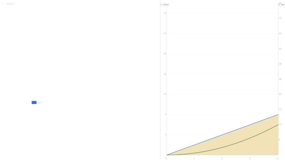
The cart starts from rest at the left end of the track and accelerates rightward at the constant rate set by the slider. At the default a = 2.0 m/s² the velocity grows by 2 m/s every second; at t = 1 s the readout shows v = 2.00 m/s, at t = 2 s it shows v = 4.00 m/s, at t = 4 s (the natural stop) it shows v = 8.00 m/s. The blue v-line on the chart is a straight ramp of slope a, anchored on the left axis whose tick marks are spaced 4 m/s apart up to a ceiling of 20 m/s (the worst-case slider value of 5 m/s² for 4 s).
Position is the integral of velocity, and for the constant-acceleration profile that integration is closed-form: x(t) = ½·a·t². With a = 2.0 m/s² the position grows quadratically; at t = 1 s the readout shows x = 1.00 m, at t = 2 s it shows x = 4.00 m, at t = 4 s it shows x = 16.00 m. The green x-curve on the chart is a parabola anchored on the right axis whose tick marks are spaced 8 m apart up to a ceiling of 40 m (the worst-case ½·5·16 = 40 m). Pause the simulation at any time and the right-axis reading of the green curve should match the Displacement readout in the controls panel exactly.
The amber-shaded triangle under the v-line is the geometric incarnation of the integral. Its area at any moment equals base · height / 2 = t · v / 2, which for v = a·t evaluates to ½·a·t²: exactly the displacement. With a = 2.0 m/s² at t = 4.00 s the triangle has base 4 s and height 8 m/s, so area = ½·4·8 = 16 m². The same number appears as the Displacement readout (16.00 m) and as the green curve's terminal value on the right axis (16 m). Three independent indicators (readout, area, and curve endpoint) all show the same value because they are all the same number reached three different ways.
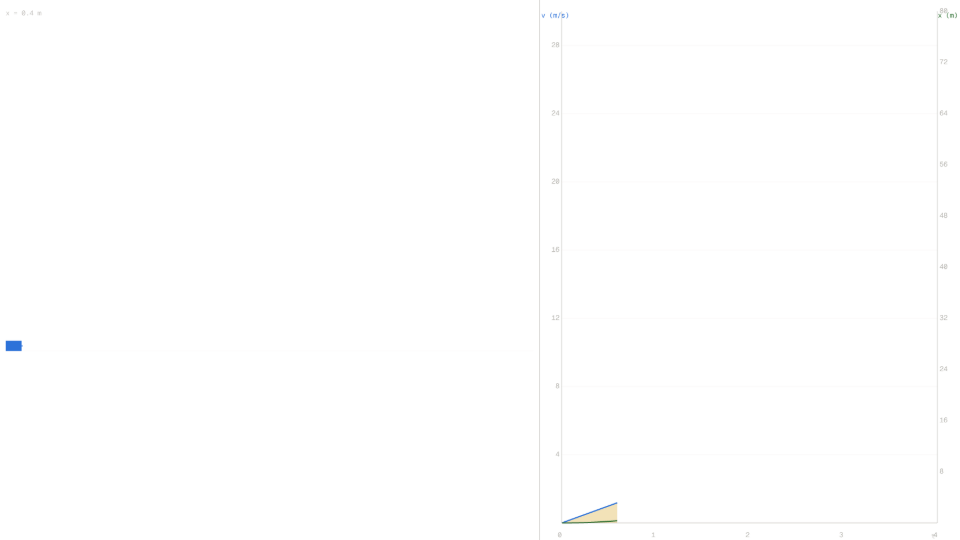
Changing the acceleration slider rescales both curves in lock-step. At a = 5.0 m/s² the v-line reaches 20 m/s at t = 4 s (the left axis ceiling) and the x-curve reaches 40 m (the right axis ceiling); at a = 0.5 m/s² the v-line barely climbs to 2 m/s and the x-curve barely climbs to 4 m. The dual-axis layout makes the rescaling proportional and visible: doubling the acceleration doubles the slope of the v-line and quadruples the displacement, exactly as v = a·t and x = ½·a·t² require.
Key Equations
For the default a = 2.0 m/s² the velocity at t = 4 s is v = 2·4 = 8.00 m/s, exactly the value the Velocity readout displays at the natural stop. The blue v-line on the chart traces this linear relationship from the origin upward at slope a: the visual signature of constant acceleration.
For the default a = 2.0 m/s² the position at t = 4 s is x = ½·2·16 = 16.00 m, exactly the value the Displacement readout displays at the natural stop. The green x-curve on the chart traces this parabolic relationship anchored on the right axis. At intermediate times the readouts can be cross-checked: at t = 2 s the predicted x = ½·2·4 = 4 m matches the Displacement readout of 4.00 m, and the green curve at that moment passes through the 4 m gridline on the right axis.
Combining the two equations above eliminates a: x = ½·t·v. With a = 2.0 m/s² at t = 4 s the right-hand side is ½·4·8 = 16 m, matching x = ½·a·t² = 16 m. This is the geometric identity the shaded triangle visualises directly: base t times height v divided by two. The simulator turns the algebraic identity into a visible area, removing any need to do the integration symbolically; it is right there on the chart.
For motion from rest, the average velocity is half of the final velocity. With the default a = 2.0 m/s² at t = 4 s the final velocity is 8 m/s and the average is 4 m/s. Multiplying average velocity by elapsed time gives the displacement: 4 m/s × 4 s = 16 m, the same value the readouts and the right axis confirm. This third path to the displacement is why area-under-the-curve and ½·a·t² are the same answer: they each integrate the same linearly rising velocity.
Key Variables
| Symbol | Name | Unit | Meaning |
|---|---|---|---|
| a | Constant acceleration | m/s² | Slider value, range 0.5 to 5 m/s²; sets the slope of the v-line |
| v(t) | Instantaneous velocity | m/s | Equals a·t starting from rest; plotted on the left axis |
| x(t) | Position from origin | m | Equals ½·a·t² starting from rest; plotted on the right axis |
| t | Elapsed time | s | Time since the run began; capped at 4 s by the natural stop |
| area | Area under v-t curve | m | Geometric displacement; equals ½·t·v at every instant |
Real World Examples
Why does an electric car's range estimate jump up the instant the driver eases off the accelerator?
The range estimate is computing the integral of velocity over time and dividing by the energy budget; both pieces depend directly on the v-t curve the car is currently tracing. While accelerating hard, the v-t line climbs steeply and the area swept under it (the displacement covered per unit energy spent) grows in proportion to ½·a·t² rather than v·t. The simulator makes this geometric distinction visible: at a = 5 m/s², the shaded triangle reaches 40 m at the natural stop t = 4 s, four times the area of the same time window at a = 1.25 m/s².
Easing off the accelerator drops the slope of the v-line, so the area accumulated per second of driving stops growing as fast, but the energy spent per second drops faster, which is why the range estimate ticks upward. The simulator's right-axis green curve is the same x = ½·a·t² that the range computer integrates from speedometer data many times per second. The dual-axis chart reproduces the exact relationship: change the slider to a smaller value and watch both the slope of the blue line and the steepness of the green parabola flatten in proportion.
How does a track-and-field coach read a sprinter's drive phase from a velocity-time tape?
Sprint coaches use velocity-time tapes from radar guns to separate the drive phase (constant acceleration off the blocks) from the maximum-velocity phase (zero acceleration). Inside the drive phase the v-t line is a straight ramp identical to the simulator's blue curve, and the area under that ramp equals the distance covered during the drive: exactly what the simulator's shaded triangle and right-axis green curve report.
With a = 5 m/s² the simulator's amber triangle area at t = 4 s is ½·4·20 = 40 m, comparable to the 30 m a top-tier sprinter covers in their first 4 s of acceleration. The coach reads the slope to grade the acceleration phase and reads the area under the curve to confirm the displacement matches the timing-gate split: two independent numbers from the same tape, exactly the dual-axis layout the simulator imposes by design. The simulator's green x-curve makes this two-number reading explicit: the slope of the blue line is one diagnostic, the height of the green curve at the same time is another, and they have to be consistent because they encode the same physics.
Why does the moon take twice as long to fall the same distance as a freely dropped rock at the lunar surface?
The lunar surface gravity gmoon ≈ 1.62 m/s² is about one-sixth of Earth's 9.81 m/s², and the kinematic identity x = ½·a·t² says falling a fixed distance takes longer in inverse proportion to the square root of acceleration. Halving the acceleration multiplies the fall time by √2, and bringing it down by a factor of six multiplies the fall time by √6 ≈ 2.45.
The simulator makes the dependency direct: at a = 1 m/s² the green x(t) curve reaches 8 m at t = 4 s, while at a = 4 m/s² it reaches 32 m at the same time, a 4× displacement ratio for a 4× acceleration ratio at fixed time. Inverting the relationship to ask how long it takes to fall a fixed distance is the standard moon-vs-Earth comparison, and the numbers come straight off the right axis of the simulator's chart. The dual-axis layout makes the v-vs-x scaling impossible to confuse: doubling the acceleration doubles the velocity at the natural stop but quadruples the displacement, and the chart shows both effects at the same instant.
Further Reading
- 1D motion plotter: the constant-velocity case, where acceleration is zero and the v-t line is flat at v₀ instead of ramped.
- Two runners position: two constant-velocity bodies on the same line, with a meeting-time formula and a 100 m finish line that ends the race.
- Free fall: constant downward acceleration g = 9.81 m/s², the same shape of v-t and x-t curves the simulator plots, just with a fixed acceleration value.
- Motion on an inclined ramp: constant acceleration g·sinθ along the slope direction, scaling the same v = a·t and x = ½·a·t² relationships by the sine of the incline angle.
- Constant-acceleration cart: the same constant-a kinematics from the body's perspective on a track, with a non-zero v₀ slider so the full x(t) = x₀ + v₀·t + ½·a·t² is on display rather than just the from-rest case.
- Average vs instantaneous velocity: the calculus limit that makes the area-under-the-curve integral exact; this article's dual-axis chart is the special case where v(t) is a straight ramp and the secant slope coincides with the tangent slope.