Variable Acceleration PhysicsIntegrate a(t) into v(t) and x(t)
Introduction
Variable acceleration describes motion in which the rate of change of velocity is itself changing with time. Unlike uniform acceleration, where a constant value of a produces a straight-line velocity graph, variable acceleration produces curved velocity and position traces whose shape depends entirely on the specific a(t) profile driving the motion.
Kinematics leans on this regime because almost every real acceleration is variable: rocket thrust builds as propellant burns off, a braking car's deceleration grows as brake pads heat, seismic ground shaking oscillates irregularly for tens of seconds. Handling these profiles requires integration, the mathematical tool that converts a(t) into v(t) and x(t).
It is tempting to assume that doubling a portion of the acceleration curve simply doubles the final speed. The integral says the effect is more subtle: the velocity gain equals the area under the entire a(t) curve, so a brief intense spike contributes the same Δv as a long gentle plateau of equal area; the shape and duration matter together, not the peak value alone.
The Physics Explained
Acceleration is defined as the time derivative of velocity: a = dv/dt. When acceleration is constant this relationship integrates trivially to v = v₀ + a·t. When acceleration varies, the integral must track every instantaneous value: v(t) = v₀ + ∫a(τ)dτ from 0 to t. The simulator evaluates this integral numerically at each time step, accumulating the product a·Δt into the running velocity total. Drawing a horizontal line at a = 2 m/s² on the acceleration canvas and pressing Run produces a v(t) graph that rises at exactly 2 m/s per second: the constant-acceleration baseline.
Position follows by a second integration: x(t) = x₀ + ∫v(τ)dτ from 0 to t. The simulator applies the same numerical step to the velocity trace it just computed, accumulating v·Δt into the running position total. This chain means that any feature drawn on the acceleration canvas propagates forward twice: first into the velocity graph, then into the position graph. A sharp upward spike in a(t) produces a steep rise in v(t) and an inflection in x(t) at the same moment.
The area interpretation is the key to reading the graphs. The velocity gained between two instants equals the signed area under the a(t) curve between those instants. A positive region adds to velocity; a negative region subtracts. Drawing a triangular pulse that rises from 0 to 4 m/s² over 3 s and then drops back to 0 (a triangle with base 3 s and height 4 m/s²) gives an area of ½·3·4 = 6 m/s, and the v(t) graph's readout at t = 3 s confirms a net gain of 6 m/s above the starting velocity.
The position graph accumulates the area under v(t) by the same logic. If the velocity rises linearly from 0 to 6 m/s over 3 s (as in the triangular-pulse example above), the area under the v(t) curve from 0 to 3 s is ½·3·6 = 9 m, and the x(t) readout at t = 3 s confirms a displacement of 9 m. Every feature of the drawn a(t) profile cascades through both integrals, making the simulator a direct visualization of the fundamental theorem of calculus applied to motion.
Key Equations
Acceleration is the rate at which velocity changes. When a(t) is not constant, this derivative takes a different value at every moment. Drawing a curve on the simulator's acceleration canvas is equivalent to specifying the value of dv/dt at every time t in the run.
Velocity at time t equals the initial velocity plus the accumulated area under the a(t) curve from 0 to t. With a triangular a(t) pulse of base 3 s and height 4 m/s² (area = 6 m/s) and v₀ = 0, the formula predicts v(3) = 0 + 6 = 6 m/s. The simulator's velocity readout at t = 3 s matches this value.
Position at time t equals the initial position plus the accumulated area under the v(t) curve. Continuing the triangular-pulse example: velocity rises linearly from 0 to 6 m/s over 3 s, giving a triangular v(t) area of ½·3·6 = 9 m. With x₀ = 0, the formula predicts x(3) = 9 m. The simulator's position readout at t = 3 s confirms this result.
The simulator advances velocity by multiplying the current acceleration value by the time step Δt and adding it to the running total. With a(t) = 2 m/s² and Δt = 0.05 s, each step adds 0.10 m/s. After 20 steps (t = 1 s) the accumulated velocity is 2.00 m/s, matching the analytical result exactly because the acceleration is constant over that segment. For a smoothly drawn curve the step errors are small and the output graph converges closely to the true integral.
Key Variables
| Symbol | Name | Unit | Meaning |
|---|---|---|---|
| a(t) | Acceleration | m/s² | Time-varying rate of change of velocity; the user-drawn input curve |
| v(t) | Velocity | m/s | Speed and direction at time t; first integral of a(t) |
| x(t) | Position | m | Displacement from origin at time t; second integral of a(t) |
| v₀ | Initial velocity | m/s | Velocity at t = 0; sets the vertical intercept of the v(t) graph |
| x₀ | Initial position | m | Position at t = 0; sets the vertical intercept of the x(t) graph |
| Δt | Time step | s | Integration interval; smaller values give higher numerical accuracy |
Real World Examples

How do engineers model the variable thrust of a rocket during launch?
A rocket's thrust is not constant: propellant burns off, atmospheric pressure drops with altitude, and engine throttle varies by mission phase. Engineers express thrust as a function of time, divide by the instantaneous mass (itself shrinking as propellant is consumed) and integrate the resulting time-varying acceleration profile to obtain velocity and position.
The Saturn V first stage produced roughly 33,000 kN at ignition, tapering over 150 s as propellant mass fell from about 2,300,000 kg to 750,000 kg, so acceleration rose from roughly 11 m/s² at liftoff to near 45 m/s² just before stage separation, a strongly non-constant profile. This is the same numerical integration the simulator performs when a non-flat curve is drawn on the acceleration canvas.
Drawing a rising ramp on the acceleration canvas, pressing Run, and reading the velocity graph produces a curve that bends upward rather than rising linearly, exactly as the Saturn V velocity trace did. The area under the drawn a(t) curve equals the final velocity shown on the v(t) graph, confirming the integral relationship at each moment of the simulated burn.
Why does a car's acceleration vary during a full-throttle run?
A car accelerating at full throttle from rest does not maintain a fixed acceleration because the engine's torque curve, gear-change events, and aerodynamic drag all evolve with speed. At low speeds drag is negligible and engine torque is near peak, so acceleration is highest. As speed rises, drag grows with the square of velocity while available engine force falls on higher gears, and acceleration declines.
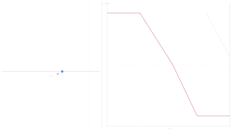
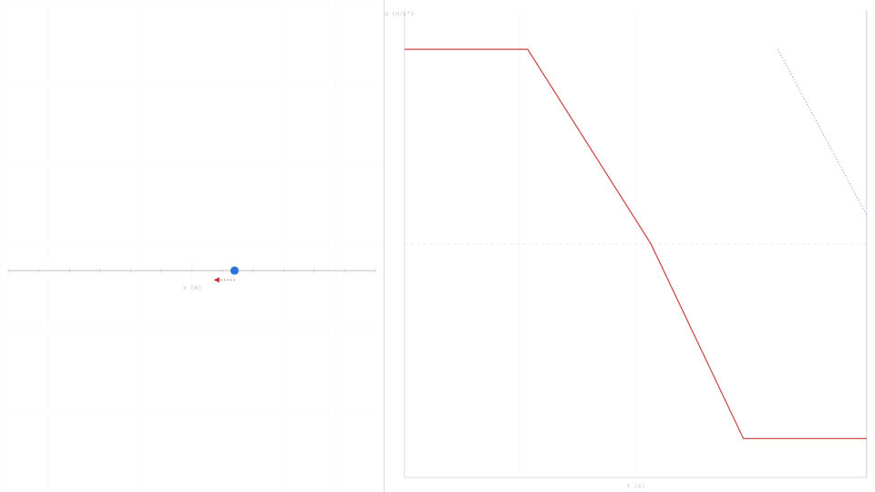
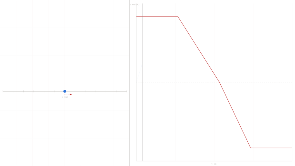
The net acceleration profile is a falling curve rather than a constant, and the resulting velocity-time graph is concave rather than linear. Drawing a smooth downward-sloping curve on the acceleration canvas (starting near 4 m/s² and ending near 1 m/s² over 10 s) and pressing Run yields a v(t) graph that rises quickly at first and then flattens, matching the character of a real vehicle's speed trace.
The position graph accumulates area under that concave velocity curve, which is why displacement grows rapidly in the first few seconds and then at a more moderate rate toward the end of the run. The simulator makes this two-stage accumulation visible in both the v(t) and x(t) panels simultaneously.
How does a seismograph record ground motion as a variable-acceleration signal?
A seismograph measures ground acceleration directly: the mass inside the instrument resists the ground's motion, and the relative displacement is proportional to ground acceleration. During an earthquake the ground acceleration record, called an accelerogram, oscillates irregularly for tens of seconds with amplitudes that rise, peak, and decay.
Structural engineers integrate that accelerogram once to get ground velocity and twice to get ground displacement, then use all three traces to evaluate how a building or bridge would respond. Drawing an oscillating, irregular curve on the acceleration canvas and pressing Run produces a velocity trace that shows the cumulative effect of each acceleration burst: a positive pulse adds area to the velocity; a negative pulse subtracts it.
With a symmetric a(t) profile that averages to zero over the full run, the simulator's v(t) graph returns toward its starting value, reproducing the net-zero-displacement constraint that well-recorded seismic events satisfy over a complete shaking cycle. The x(t) panel then shows the ground's net displacement history as the double integral of the drawn profile.
Further Reading
- Elastic collisions: conservation of momentum and kinetic energy in two-body impacts; a contrasting case where the key quantity is impulse rather than a time-varying integral.
- Projectile motion: two-dimensional kinematics under constant gravitational acceleration; the baseline for understanding why variable acceleration produces qualitatively different trajectories.
- Constant-acceleration cart: the special case where a is constant, reducing the numerical a(t)→v(t)→x(t) integration chain to the closed-form v = v₀ + a·t and x = v₀·t + ½·a·t².
- Velocity-time plotter: the constant-a case from the dual-axis chart perspective; this article's a(t)→v(t)→x(t) cascade reduces to the v-t plotter's blue ramp + green parabola when the drawn a(t) is flat.
- Two runners position: the simplest case (a = 0), where the a(t) input curve would be flat at zero and the integration chain collapses to two linear x(t) lines whose intersection gives the meeting time.
- Average vs instantaneous velocity: the calculus limit definition that underlies the numerical integration scheme; the Euler step v(t+Δt) ≈ v(t) + a(t)·Δt is the same average-velocity-over-Δt construction at the heart of this article.