Simulation

Variable Acceleration

KinematicsAcceleration

Adjust a peak-acceleration slider to shape a piecewise-linear acceleration-time profile; the simulation integrates it in real time to reveal velocity and position — the graphical meaning of kinematic integration.

Objective

Verify that the area under a piecewise-linear acceleration-time curve equals the change in velocity, and that the area under the resulting velocity-time curve equals displacement. The model treats the particle as a point mass in one dimension with no drag and no boundary; acceleration follows a hardcoded symmetric profile scaled by the peak-acceleration slider.

Setup

Leave the Peak acceleration slider at its default of 5 m/s² and press Start. The particle begins at rest: x = 0, v = 0.
Watch the Velocity (m/s) readout for the first 4 seconds — it should climb at a steady 5 m/s² while the profile segment is flat.
At t = 4 s, note v and x from the HUD. Predicted: v ≈ 20 m/s, x ≈ 40 m.
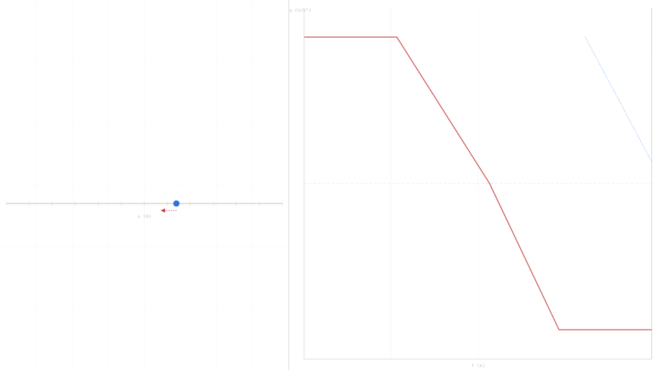
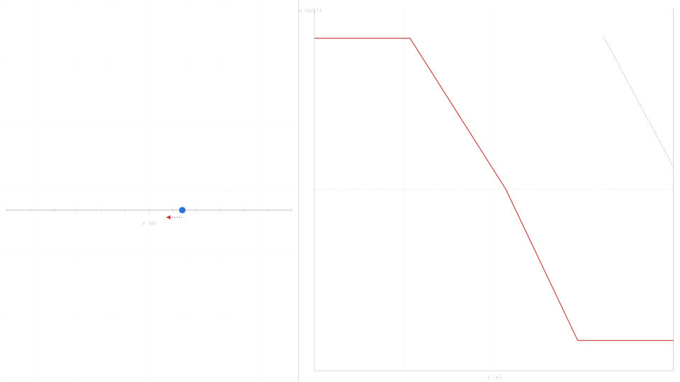
Let the run continue to t = 15 s. The acceleration ramps to −5 m/s² after t = 8 s, so velocity peaks near t = 8 s then decreases.
Press Reset, set Peak acceleration to 10 m/s², and repeat — all velocity and position values should double.

Analytical Prediction

With the default profile (a = 5 m/s² for 0 ≤ t ≤ 4 s), constant-acceleration kinematics give:

v(4)=v₀ + a · t

=0 + 5 · 4

=20 m/s

x(4)=x₀ + v₀ · t + ½ · a · t²

=0 + 0 + ½ · 5 · 16

=40 m

Between t = 4 s and t = 8 s, a drops linearly from 5 to 0 m/s². The velocity increment equals the triangular area: Δv = ½ · 5 · 4 = 10 m/s, so v(8) ≈ 30 m/s. After t = 8 s the acceleration is negative and velocity decreases symmetrically back toward zero.

Results Analysis

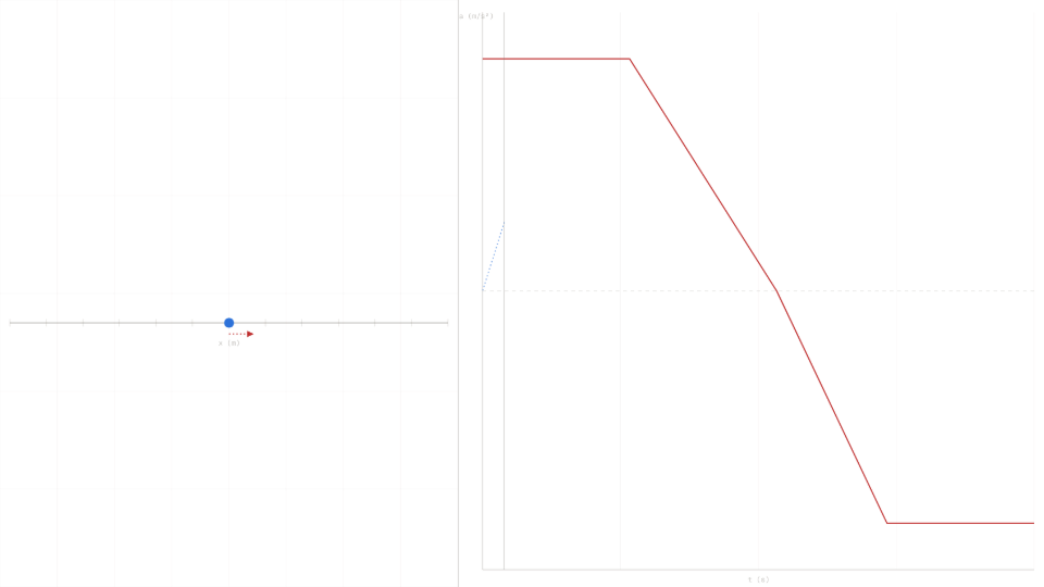
Compare the Velocity (m/s) readout at t = 4.00 s to the predicted 20 m/s — typical agreement is within 0.1 m/s at the default substep rate. The Position (m) readout should read near 40 m at the same instant. Confirm the Acceleration (m/s²) readout matches the profile value at each segment boundary: 5 at t = 0, transitioning to 0 at t = 8 s, and −5 at t = 11 s. The right-panel graph overlays the a(t) profile in red and the running velocity trace in blue — the area-equals-velocity-change relationship is visible as the filled region between the profile and the time axis.

Source of Error

The model is a one-dimensional point-mass integrator — no drag, no gravity projection, no rotational inertia, and no track boundary. The piecewise-linear profile is exact between control points; only the Euler integration step introduces numerical error. The analytical prediction in the Setup section uses the same idealized piecewise-linear profile and the same constant-acceleration formulas, so the physical idealizations cancel between prediction and simulation. The residual gap between the predicted 20 m/s and the displayed readout is therefore purely numerical, not physical, for this sim.

Further Exploration

Set Peak acceleration to 1 m/s² and run to t = 4 s — does the velocity readout show approximately 4 m/s? This confirms proportional scaling between peak acceleration and peak velocity.
What happens to the final position when you double the peak to 10 m/s²? Predict the ratio before running — does the sim confirm that position scales as the square of peak acceleration during the constant segment?
The profile is symmetric: equal positive and negative phases. Does the particle return to x = 0 by t = 15 s? Why or why not — what does the velocity trace on the right panel tell you?
Pause the simulation at exactly t = 8 s using the Pause button and read the velocity. Compare it to the area under the a(t) curve from t = 0 to t = 8 s visible on the right-panel graph.