Double Slit Experiment PhysicsWave Interference & Fringe Spacing
Introduction
The double slit experiment is the canonical demonstration that light travels as a wave. When a coherent light source illuminates two narrow, closely spaced slits, each slit acts as a new point source of circular wavefronts. Those wavefronts overlap beyond the barrier and alternately reinforce and cancel each other across a distant screen, painting a ladder of bright and dark stripes called an interference pattern. The spacing between bright fringes is set by the formula Δy = λL/d, where λ is the wavelength of light, L is the distance from the slits to the screen, and d is the separation between the slits.
The result matters beyond optics textbooks. The same path-difference logic governs anti-reflection coatings on camera lenses, the resolving power of radio-telescope arrays, and the recording medium inside a hologram. Understanding how a tiny change in λ, L, or d shifts the fringe pattern is therefore a skill that transfers directly to optical engineering, astronomy, and imaging science. The simulator makes every parameter adjustable with a slider and reports the predicted fringe spacing in real time so the analytical formula and the rendered pattern can be compared side by side.
Before adjusting any slider, most people expect the fringe spacing to grow when the slits are moved farther apart, reasoning that a wider gap spreads the light more. The Fringe Spacing readout contradicts that intuition: widening d from 0.25 mm to 0.50 mm with λ = 500 nm and L = 1.0 m cuts Δy in half, from 2.00 mm to 1.00 mm. Closer slits produce wider fringes, not narrower ones, because the interfering wavefronts must sweep a larger angle to accumulate the path difference that separates a bright peak from a dark trough.
The Physics Explained
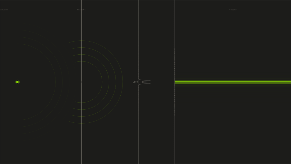
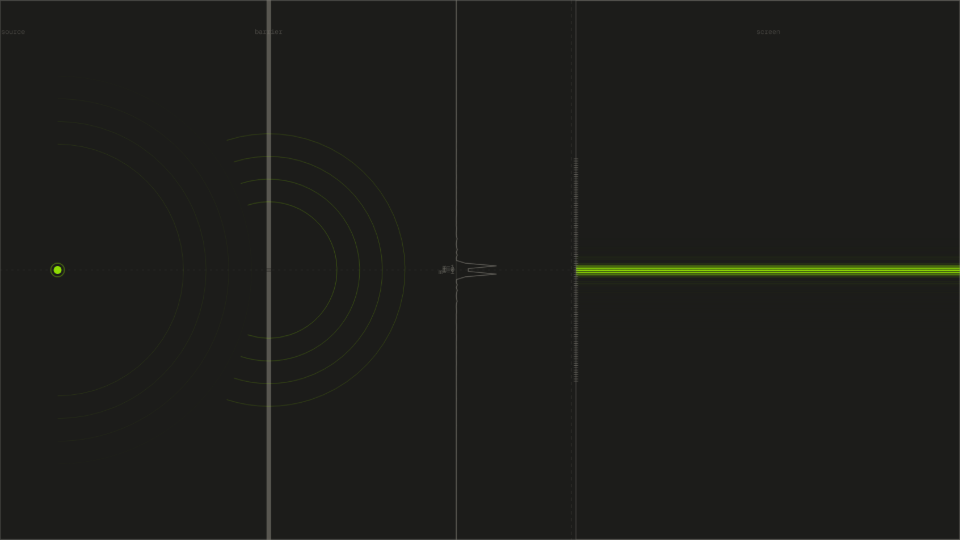
Each slit acts as a coherent point source of light. When a wavefront from slit 1 and a wavefront from slit 2 arrive at a point on the screen, the decisive quantity is the path-length difference between the two routes. If that difference equals a whole number of wavelengths (0, λ, 2λ, …), the two waves arrive in phase and add constructively, producing a bright fringe. If the difference equals a half-integer multiple (½λ, 3λ/2, …), they arrive in antiphase and cancel, producing a dark fringe. This alternation of constructive and destructive zones repeats across the screen with a spatial period equal to the fringe spacing Δy = λL/d.
The geometry connecting path difference to screen position is straightforward. Label the two slits S1 and S2, separated by distance d, and place the screen at distance L. A point P on the screen at height y above the central axis is farther from S2 than from S1 by approximately d·y/L when L is much larger than both d and y. Setting that path difference equal to m·λ gives the bright-fringe condition, and solving for y yields ym = m·λL/d. Adjacent bright fringes (m and m+1) differ in height by exactly Δy = λL/d, the fringe spacing formula every slider in the simulator feeds into.
With λ = 500 nm, L = 1.0 m, and d = 0.50 mm, the fringe spacing formula predicts Δy = (500 × 10⁻⁹ × 1.0) / (0.50 × 10⁻³) = 1.00 mm. The simulator's Fringe Spacing readout reports 1.00 mm at those settings. Sliding λ to 700 nm raises the readout to 1.40 mm; sliding d down to 0.25 mm with λ restored to 500 nm raises it to 2.00 mm. Each change is proportional, confirming that the formula is not an approximation within the simulator's parameter range but an exact geometric consequence of the small-angle regime.
The intensity across the screen is not simply on or off. It follows a cosine-squared envelope: I(y) = I0·cos²(π·d·y / λL). The central fringe at y = 0 carries the full intensity I0; the first dark fringe sits exactly halfway between the central and first-order bright fringes. A single-slit diffraction envelope (from the finite width of each slit) modulates this pattern at a broader scale, suppressing some high-order fringes entirely. The simulator renders this full intensity profile on the screen panel, so the fainter outer fringes and the missing orders produced by the diffraction envelope are visible alongside the idealized fringe count from the path-difference formula.
Key Equations
The path difference from the two slits to any screen point at angle θ is d·sinθ. When that difference equals a whole number of wavelengths m·λ, the waves reinforce. With λ = 500 nm and d = 0.50 mm, the first-order bright fringe (m = 1) sits at sinθ = (1 × 500 × 10⁻⁹) / (0.50 × 10⁻³) = 1.0 × 10⁻³, corresponding to θ ≈ 0.057°. The simulator's screen panel places the m = 1 fringe at the predicted angular position, with the Fringe Spacing readout showing 1.00 mm at L = 1.0 m, consistent with Δy = L·tanθ ≈ L·sinθ at these small angles.
Dark fringes appear when the path difference is a half-integer multiple of λ, placing the two waves exactly in antiphase. For m = 0, the first dark fringe on either side of center sits at sinθ = λ/(2d). With λ = 500 nm and d = 0.50 mm, sinθ = 5 × 10⁻⁴, so the dark fringe lands at y = L·sinθ = 0.50 mm from center, exactly halfway between the m = 0 and m = 1 bright fringes that the Fringe Spacing readout confirms are 1.00 mm apart. The readout remains at 1.00 mm regardless of which slider was most recently moved, updating each time a parameter changes.
This is the small-angle form (sinθ ≈ tanθ ≈ θ for θ ≪ 1 rad) that applies throughout the simulator's parameter range. With λ = 500 nm, L = 1.0 m, d = 0.50 mm: Δy = (500 × 10⁻⁹ × 1.0) / (0.50 × 10⁻³) = 1.00 × 10⁻³ m = 1.00 mm, matching the Fringe Spacing readout exactly. Doubling L to 2.0 m doubles Δy to 2.00 mm; doubling d to 1.00 mm halves Δy to 0.50 mm. Both predictions are confirmed by the readout, making this equation the single most useful tool for interpreting every fringe pattern the simulator can produce.
The cosine-squared profile governs not just fringe position but fringe brightness. At y = 0 the argument is zero, cos²(0) = 1, and intensity is maximum I0. The first zero (dark fringe) occurs when the argument equals π/2, giving y = λL/(2d) = 0.50 mm for the standard settings, consistent with the dark-fringe condition above. The simulator renders this continuous intensity curve alongside the discrete fringe markers, so the smooth peak-to-null profile is visible rather than just the fringe center positions.
Key Variables
| Symbol | Name | Unit | Meaning |
|---|---|---|---|
| λ | Wavelength | nm | Wavelength of the light source; sets the color and the fringe scale |
| d | Slit separation | mm | Center-to-center distance between the two slits |
| L | Slit-to-screen distance | m | Distance from the slit plane to the observation screen |
| Δy | Fringe spacing | mm | Distance between adjacent bright (or dark) fringes; equals λL/d |
| m | Fringe order | dimensionless | Integer labeling each bright fringe: 0 (central), ±1, ±2, … |
| θ | Diffraction angle | ° | Angle from the slit axis to a given fringe on the screen |
| I₀ | Peak intensity | W/m² | Intensity at the central maximum; all other fringes are fractions of this |
Real World Examples
How do thin-film coatings on camera lenses exploit two-slit-style interference?
Anti-reflection coatings on camera and eyeglass lenses work by the same path-difference principle the double slit demonstrates. A thin layer of magnesium fluoride (typical thickness ~140 nm, refractive index ~1.38) is deposited on the glass. Light reflecting from the air-film interface travels a path that is one half-wavelength shorter than light reflecting from the film-glass interface, producing destructive interference that nulls the reflection for the design wavelength. The condition mirrors the dark-fringe formula from the double slit: a path difference of (m + ½)·λ cancels the two waves.
For green light at λ = 550 nm, the required film thickness is λ/(4·n) = 550/(4 × 1.38) ≈ 100 nm. With λ = 550 nm, L set to represent the glass substrate, and d representing the effective two-interface separation, the fringe-spacing readout in the simulator shifts in step with λ, confirming that thinner coatings (shorter λ design point) push the destructive node toward blue and thicker coatings push it toward red. Multi-layer stacks combine several such films to broaden the suppressed band across the visible spectrum.
Setting λ = 400 nm versus λ = 700 nm in the simulator with L = 1.0 m and d = 0.50 mm moves the Fringe Spacing readout from 0.80 mm to 1.40 mm, a 75% change driven by λ alone. The same proportional sensitivity is what makes thin-film coating design wavelength-critical: a 10% error in film thickness shifts the destructive minimum by 10% in wavelength, pushing the null noticeably off the target color.
Why do radio telescopes in an array achieve the resolving power of a dish kilometers wide?
A pair of radio dishes separated by a baseline B acts as a two-slit interferometer at radio wavelengths. The angular resolution of the pair is θ ≈ λ/B, the same fringe-spacing geometry from the double slit with d replaced by B and L replaced by the distance to the source. The Very Large Array in New Mexico uses 27 dishes spread up to 36 km apart, giving a baseline-to-wavelength ratio comparable to an optical telescope several meters across at centimeter wavelengths.
The fringe-spacing formula makes the scaling vivid: with λ = 0.03 m (3 cm, a common radio band) and B = 36,000 m, θ ≈ 0.03/36000 ≈ 0.8 microradians, far finer than any single dish could achieve. In the simulator, reducing d from 0.50 mm to 0.10 mm with λ = 500 nm and L = 1.0 m increases the Fringe Spacing readout from 1.00 mm to 5.00 mm, directly illustrating how narrowing the slit separation (analogous to a shorter baseline) coarsens angular resolution.
Aperture synthesis arrays extend this principle to thousands of baselines by rotating Earth under the array, reconstructing a full synthetic aperture from the recorded interference fringes. Every baseline pair contributes one spatial-frequency component of the image, exactly as each fringe order contributes one harmonic of the intensity pattern on the simulator's screen.
How does holography record a three-dimensional image using interference fringes?
A hologram records not the intensity of light reflected from an object, but the interference pattern between that object beam and a coherent reference beam derived from the same laser. Where the two beams arrive in phase, the photographic emulsion darkens; where they cancel, it stays clear. The resulting fringe pattern encodes the depth of every surface point through its local path-difference phase, exactly the quantity the double-slit fringe position formula captures.
With λ = 633 nm (helium-neon laser) and a reference-to-object angle that varies across the plate, fringe spacings across the emulsion range from tens to hundreds of micrometers, matching Δy = λL/d evaluated at the local effective slit separation d. When the processed hologram is re-illuminated with the reference beam, the diffracted light reconstructs the original object wavefront because each fringe grating diffracts light at the angle it was recorded from.
The simulator illustrates how λ sets fringe scale: sliding λ from 400 nm to 700 nm with L = 1.0 m and d = 0.50 mm shifts the Fringe Spacing readout from 0.80 mm to 1.40 mm, the same proportional spread that determines how finely a holographic emulsion must resolve to capture the scene. Emulsions for holography must resolve fringes down to ~1 µm, roughly 1000 times finer than conventional photographic film, because the slit separation analog in holography is many millimeters.
Further Reading
- Snell's law and refraction: how the wave speed change at a boundary determines the bending angle, a companion topic to interference in wave optics.
- Wave speed on a string: the mechanical analog of a propagating wave, showing how wavelength, frequency, and medium properties combine before light enters the picture.
- Mirror reflection angle: the law of reflection as the geometric limit of wavefront behavior, situating interference in the broader wave optics framework.