Simulation

Spring Potential Energy · SimulatorU = ½kx², the quadratic energy curve

Energy & WorkPotential energy

Compress or stretch a spring; PE rises quadratically with displacement, with U-vs-x graph alongside

Published: July 3, 2026

Objective

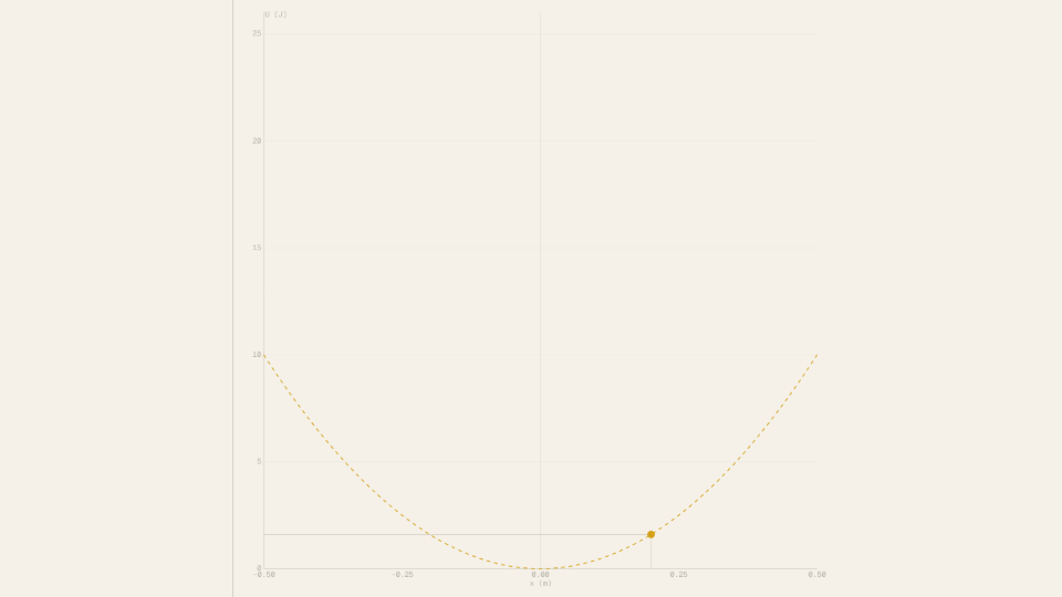
Verify that elastic potential energy obeys U = ½kx² by compressing and stretching a spring across the full slider range, comparing the live U readout against the analytical formula, and observing the parabolic U-vs-x curve. The spring is ideal (massless, Hookean) and the tug animation uses a fixed representative mass for visual effect only.

Setup

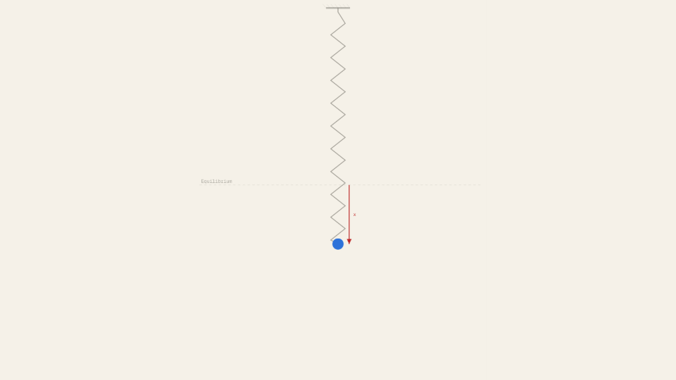
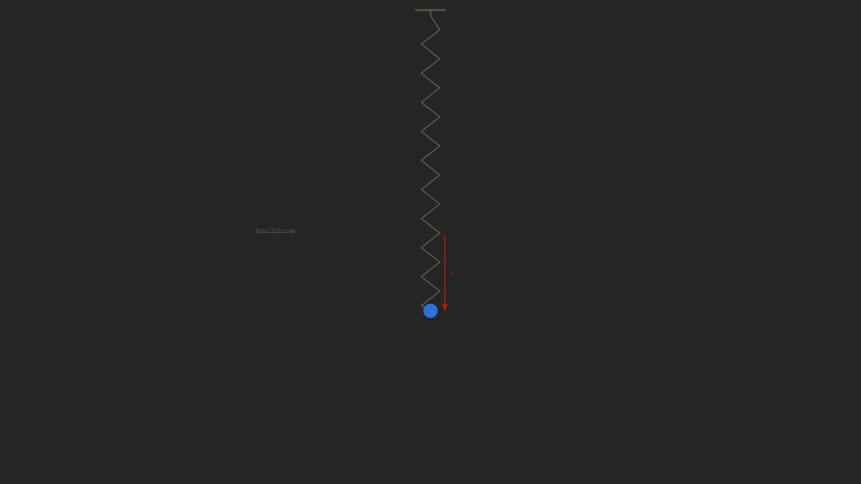
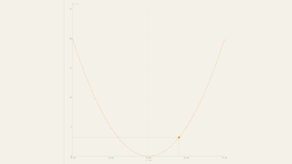
Set the Spring Constant slider to k = 80 N/m (default) and the Displacement slider to x = 0.20 m. Observe the spring coil stretch and note U = 1.60 J in the readout. The U-vs-x parabola and the amber dot are already visible.
Press Start. Watch the body oscillate once and settle to x = 0.20 m. Confirm the final U readout matches 1.60 J (formula: ½ × 80 × 0.20² = 1.60 J).
Press Reset. Move the Displacement slider to x = 0.40 m. Before pressing Start, predict U: it should be 4 × 1.60 = 6.40 J (x doubled, U quadrupled). Press Start and verify.
Press Reset. Move the Spring Constant slider to k = 160 N/m, keep x = 0.20 m. Predict U = ½ × 160 × 0.04 = 3.20 J (double k, double U at same x). Press Start and confirm.
Press Reset. Set x = −0.20 m (compression). Press Start and record U. Compare to the +0.20 m result to confirm the symmetry U(−x) = U(+x).
Press Reset. Set x = 0 m. Press Start and verify U = 0.000 J and F = 0.00 N — the spring at its natural length stores no energy.

The spring stretched to x = 0.20 m from equilibrium, with the displacement arrow and coil visible before starting.

The U-vs-x parabola for k = 80 N/m with the live dot at x = 0.20 m, U = 1.60 J, showing the quadratic shape.

A stiffer spring (k = 160 N/m) produces a narrower, steeper parabola; the same x = 0.20 m displacement now stores U = 3.20 J.

Analytical Prediction

The elastic potential energy formula is U = ½kx². With k = 80 N/m and x = 0.20 m:

U=½ · k · x²

=½ · 80 · 0.20²

=½ · 80 · 0.04

=1.60 J

Doubling the displacement to x = 0.40 m gives:

U=½ · 80 · 0.40²

=½ · 80 · 0.16

=6.40 J

This is exactly 4 × 1.60 J, confirming the quadratic relationship. The spring force at x = 0.20 m is F = −kx = −80 × 0.20 = −16.0 N (restoring, opposing extension). At x = 0 the energy and force are both zero, placing the dot at the vertex of the parabola.

Results Analysis

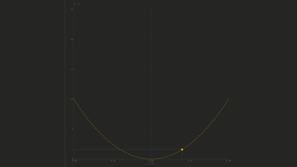
After each run settles, read the Potential Energy (J) readout labeled uOut and compare to the formula ½kx² using the slider values shown in the Spring Constant (N/m) readout kOut and the Displacement (m) readout xOut. At k = 80 N/m, x = 0.20 m, the readout should show 1.600 J within 0.010 J of the analytical value. At x = 0.40 m the readout should show 6.400 J, demonstrating the 4:1 ratio. On the U-vs-x graph the amber dot tracks the current (x, U) coordinate; cross-hair guides connect the dot to both axes, reinforcing the readout values. The reference parabola redraws when the k slider changes, showing the curvature increase for stiffer springs.

Source of Error

This simulation models an ideal, massless Hookean spring with no coil binding, no material fatigue, and no elastic limit. Real springs deviate from F = −kx at large deformations and possess distributed mass that stores kinetic energy in the coil itself. The tug animation uses a fixed representative mass (1 kg) and a prescribed damping ratio for visual effect only, not to model the true dynamic response of any physical spring-mass system. No gravity acts on the bob in the energy calculation. Because the analytical formula and the simulation use the same ideal model, any residual between the predicted and displayed U values is numerical only, not physical.

Further Exploration

Set x = 0.10 m and record U, then set x = 0.20 m and record U again. Is the second value exactly 4 × the first? Try x = 0.30 m and x = 0.40 m to see whether the 4× pattern continues along the parabola.
Keep x fixed at 0.20 m and sweep k from 10 to 200 N/m. How does the parabola curvature change? At what k does U exceed 4 J for x = 0.20 m? (Answer: k > 200 N/m, confirming 4 J requires k = 200 N/m.)
Set x = −0.50 m (maximum compression) and x = +0.50 m (maximum extension). Are the U readouts equal? What does this symmetry imply about the sign of displacement in energy storage?
Set x = 0 m and press Start. What do the U, F, and x readouts show? Why is this configuration the minimum-energy state of the spring, and what would it take to move the dot away from the parabola vertex?
Run three successive experiments at x = 0.20 m, x = 0.30 m, and x = 0.40 m without pressing Clear. Can you see the ghost dots on the parabola from previous runs? What pattern do their U values trace?