Simulation

Impulse from a Force Pulse · SimulatorImpulse equals area under the force-time curve

Momentum & CollisionsImpulse

A cart hit by a force pulse with adjustable magnitude and duration; impulse equals area under force-time curve

Published: August 17, 2026

Objective

Verify the impulse-momentum theorem by observing that the shaded area of the force-time rectangle equals the cart's change in momentum, regardless of how force and pulse duration are individually varied. The simulation assumes a frictionless, horizontal track and a perfectly rectangular force pulse, so the only variable affecting momentum is J = F·Δt.

Setup

Set Force F = 40 N, Pulse Duration Δt = 0.5 s, and Cart Mass m = 1.0 kg (all defaults). Note the impulse J shown in the readout before pressing Start.
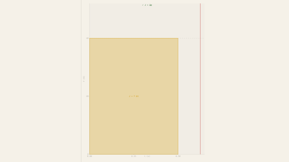
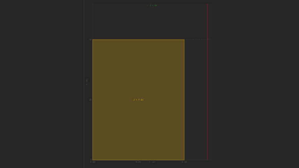
Press Start and observe the cart accelerate during the pulse, then coast at constant velocity. Watch the amber rectangle on the force-time graph fill in as the cursor sweeps to t = 0.5 s, then stops.
Record the Impulse J (N·s), Δp (kg·m/s), and Velocity v (m/s) readouts once the run finishes. Confirm that J ≈ Δp ≈ m × v = 1.0 × 20.0 = 20.0.
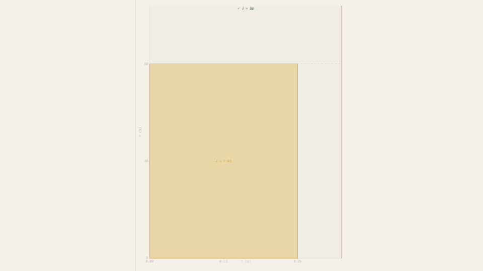
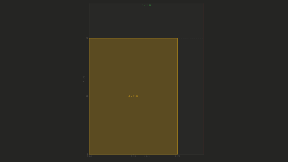
Press Reset, change Force to 80 N and Pulse Duration to 0.25 s (keeping m = 1.0 kg). Press Start again. Compare the new rectangle on the graph with the grey ghost rectangle from the previous run.
Press Reset, change Cart Mass to 2.0 kg with F = 40 N and Δt = 0.5 s. Press Start. Note that J remains 20.0 N·s but v drops to 10.0 m/s, confirming J = Δp = m·v with a heavier cart.

The cart sits at rest on a frictionless track before the force pulse begins, with sliders set to F = 40 N, Δt = 0.5 s, and m = 1 kg.

The force-time graph after the pulse completes: the shaded amber rectangle has area J = 20 N·s, which equals the cart's momentum change Δp = m·v = 20 kg·m/s.

Doubling F and halving Δt gives the same area (J = 20 N·s) and the same final speed, shown as a ghost rectangle from the prior run alongside the new taller, narrower rectangle.

Analytical Prediction

With the default values F = 40 N, Δt = 0.5 s, and m = 1.0 kg, the impulse-momentum theorem predicts:

J=F·Δt

=40 × 0.5

=20.0 N·s

The cart starts at rest, so v_initial = 0 and the momentum change equals the impulse:

Δp=m·v_final − m·v_initial

=1.0 × v_final − 0

=20.0 kg·m/s

Solving for v_final:

v_final=J / m

=20.0 / 1.0

=20.0 m/s

For the second run (F = 80 N, Δt = 0.25 s, m = 1.0 kg), the rectangle is taller and narrower but the area is identical: J = 80 × 0.25 = 20.0 N·s, so v_final = 20.0 m/s again. The same-impulse result, visible as equal-area rectangles on the graph, is the core insight of this sim.

Results Analysis

After each run, check that the Impulse J readout shows 20.00 N·s (analytically computed from the sliders, not integrated), the Δp readout approaches 20.00 kg·m/s, and the Velocity v readout approaches 20.00 m/s. The forest-green badge on the graph confirms J ≈ Δp once the run finishes. For the mass-variation run (m = 2.0 kg), J remains 20.00 N·s while v drops to approximately 10.00 m/s and Δp stays near 20.00 kg·m/s. The ghost rectangle from the first run and the live rectangle from the second run share the same area on the graph, visually confirming that a different force-duration combination can deliver identical impulse.

Source of Error

The primary idealizations are a frictionless horizontal track and a perfectly rectangular force pulse. Real cart experiments involve rolling friction and a force that rises and falls over the contact time rather than switching on and off instantaneously. The simulation integrates the constant acceleration using small fixed time steps, so the final velocity after the pulse differs from the analytical F·Δt/m by a small Euler-integration error, typically under 1% for the default slider settings. Both the analytical prediction and the sim share the rectangular-pulse assumption, so this idealization cancels out in the comparison. The residual gap between the Δp readout and the J readout is therefore purely numerical, not physical.

Further Exploration

Set F = 20 N and Δt = 1.0 s, then run. Next set F = 80 N and Δt = 0.25 s. Do the Impulse and Velocity readouts agree? What shape difference appears between the ghost and live rectangles on the graph?
Keep J fixed by always setting F × Δt = 20 N·s. How many different (F, Δt) pairs can you find that give the same final speed? What does this tell you about which physical quantity actually governs the outcome?
Set Cart Mass to its minimum (0.5 kg) and its maximum (5.0 kg) with the same F = 40 N and Δt = 0.5 s. How does the cart's final velocity scale with mass? Does the Impulse J readout change?
Set Pulse Duration to its minimum (0.05 s) and Force to its maximum (100 N). Describe the motion: does the cart still coast after the pulse ends? What is the predicted v_final?
After two or three runs with different settings, look at the ghost rectangles accumulated on the graph. Can you find a combination where the live rectangle and a ghost rectangle have the same area but clearly different shapes? What does that mean for J and Δp?