Wave Speed on a String · SimulatorWave Speed Formula v = √(T/μ)
Adjust string tension and linear density; pulse speed varies as √(T/μ)
Published: June 19, 2026
Objective
Verify that the wave speed formula v = √(T/μ) produces a square-root (sublinear) relationship between tension and pulse speed on a stretched string. The simulation models a transverse pulse bouncing on an ideal, massless-outside-the-pulse string with fixed endpoints, assuming no energy dissipation, no dispersion, and no standing-wave buildup.
Setup
- Leave the sliders at their defaults (Tension 20 N, Linear Density 0.020 kg/m) and read the Wave Speed readout before pressing Start. Record the displayed value.
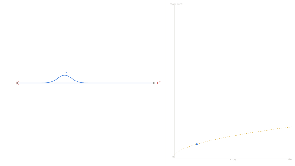
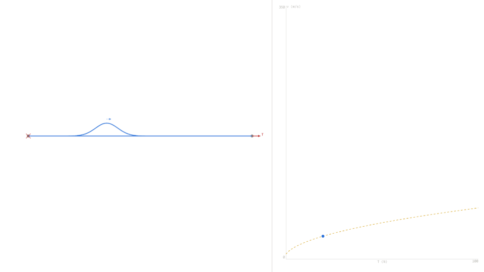
- Press Start. Watch the Gaussian pulse traverse the 8 m string and count each reflection as the Bounces readout increments. Note that the Wave Speed readout stays constant throughout the run.
- After the run completes (5 bounces), press Reset. Change Tension to 80 N (keep Linear Density at 0.020 kg/m). Record the new Wave Speed shown in the readout before pressing Start.
- Press Start again. Observe that the pulse crosses the string faster. Compare the new speed to the first run and note that 4× the tension gives roughly 2× the speed, not 4×.
- Reset, then change Linear Density to 0.005 kg/m (keep Tension at 20 N). Record the predicted speed and Start. Observe the same doubling effect from halving the denominator.
Analytical Prediction
The formula v = √(T/μ) predicts the following values for the three configurations in the setup. Default (T = 20 N, μ = 0.020 kg/m):
High tension (T = 80 N, μ = 0.020 kg/m):
Ratio 63.2 / 31.6 ≈ 2.00, confirming that quadrupling tension doubles speed (√4 = 2, not 4). Low density (T = 20 N, μ = 0.005 kg/m):
Halving the denominator (from 0.020 to 0.005 is a factor of 4) also doubles speed by the same square-root law. The v(T) graph in the secondary panel shows the concave-down curve characteristic of a square-root function, where each additional newton of tension yields a smaller speed gain than the previous one.
Results Analysis
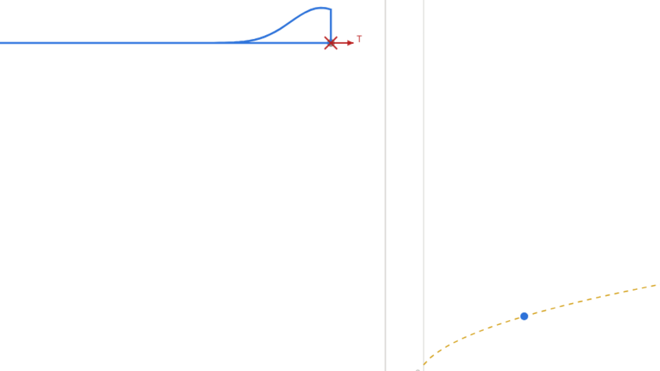
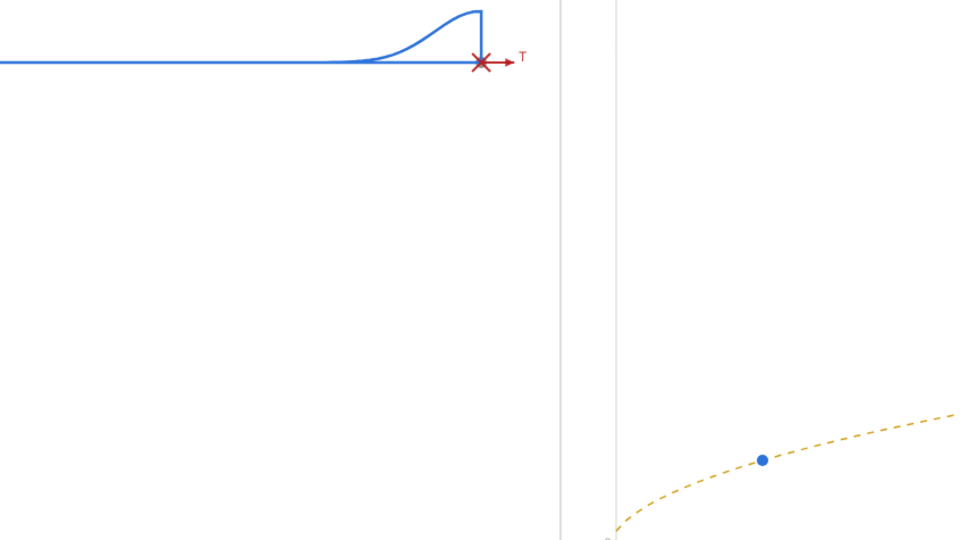
After each run, compare the Wave Speed readout in the HUD to the predicted value from the formula. At defaults (T = 20 N, μ = 0.020 kg/m) the readout should show 31.6 m/s within ±0.1 m/s of the exact value 31.623 m/s. At T = 80 N, μ = 0.020 kg/m the readout should show 63.2 m/s (exact 63.246 m/s). Verify that the Bounces counter increments each time the pulse reaches an endpoint and that the time at which the 5th bounce occurs matches the prediction t_stop = 5 × 2 × 8 / v (approximately 2.53 s at defaults). The v(T) operating point (sky dot) in the secondary panel should sit on the amber dashed reference curve at the correct (T, v) coordinates for each slider combination. The speed readout must not change during a run, confirming there is no numerical drift or dispersion in the integration.
Source of Error
The model assumes an ideal string with uniform linear density, perfectly rigid endpoints, and no energy loss at reflections. In a real string, slight stiffness (bending rigidity) causes dispersion so shorter wavelengths travel faster than predicted by the simple formula. Real end-fixtures absorb a fraction of wave energy each bounce, reducing amplitude. The linear density of a real string varies slightly along its length due to manufacturing tolerances. This simulation also treats the pulse as a point position in the physics layer (the Gaussian envelope is purely visual), so any amplitude-dependent effects such as nonlinear string stretching are absent. Because both the model and the analytical prediction share these idealizations, the residual gap between the displayed readout and the formula value is purely numerical, not physical.
Further Exploration
- Find the tension needed to double the default speed (≈ 63.2 m/s) at μ = 0.020 kg/m. Is it 40 N (2×) or 80 N (4×)? Why does the answer reveal the square-root law?
- Set T = 5 N and μ = 0.005 kg/m. Predict and verify that the speed equals the default (T = 20 N, μ = 0.020 kg/m) result. What ratio of T to μ produces identical speeds?
- Drag μ from 0.001 to 0.100 kg/m in Fresh state and watch the v(T) reference curve in the secondary panel rescale. At μ = 0.001 kg/m the curve is much steeper — why does a lighter string respond more strongly to the same tension increase?
- At T = 1 N and μ = 0.100 kg/m the pulse moves at only about 3.2 m/s. How many seconds does it take to complete 5 traversals on the 8 m string? Does the sim reach the bounce limit or the 15 s time cap?
- Compare two runs: T = 40 N, μ = 0.040 kg/m versus T = 20 N, μ = 0.020 kg/m. Are the ghost trails from both runs the same length in the same time window? What does this tell you about equal-speed combinations?