Average vs Instantaneous Velocity SimulatorSecant vs Tangent Slope
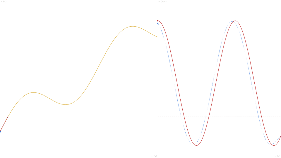
A position-time curve with a draggable secant line that shrinks to a tangent, illustrating the limit definition of instantaneous velocity.
Published: May 10, 2026 · Updated: May 28, 2026
Objective
Verify the limit definition of instantaneous velocity by observing how a secant line on a position-time curve approaches the tangent as the time interval Δt shrinks toward zero. The curve follows x(t) = 3·sin(0.5·t) + 0.8·t (a deliberately non-uniform motion), so neither the average nor the instantaneous velocity is constant, making the distinction between the two measurable and vivid.
Setup
- Set the Interval Δt slider to 2.0 s. Press Start and let the simulation run for about 5 seconds, then press Pause. Record the Avg Velocity and Inst Velocity readouts.
- Press Reset. Set Δt to 1.0 s. Press Start, advance to roughly the same simulation time (~5 s), and pause. Record both velocity readouts and note how the two values have moved closer together.
- Repeat with Δt = 0.05 s, the minimum value. The blue dashed secant on the position-time plot should nearly coincide with the red tangent line, and the two velocity readouts should differ by less than 0.05 m/s.
- While in Fresh state, sweep the Δt slider slowly from 2.0 s down to 0.05 s and watch the blue dashed secant rotate toward the red tangent in real time on the left panel.
Analytical Prediction
The position function is x(t) = 3·sin(0.5·t) + 0.8·t, so the instantaneous velocity is its derivative: v(t) = 1.5·cos(0.5·t) + 0.8. At t = 5 s the instantaneous velocity is:
The average velocity over [5, 7] s (Δt = 2 s) is (x(7) − x(5)) / 2. With x(5) = 3·sin(2.5) + 4 ≈ 5.80 m and x(7) = 3·sin(3.5) + 5.6 ≈ 4.55 m:
As Δt shrinks to 0.05 s, v̄ converges to v(5) ≈ −0.40 m/s. The two readouts should agree to within ±0.02 m/s at the minimum slider setting.
Results Analysis
While the simulation is paused near t ≈ 5 s, compare the Avg Velocity (m/s) and Inst Velocity (m/s) readouts for each Δt setting. With Δt = 2.0 s the readouts should show roughly −0.62 m/s and −0.40 m/s respectively, a gap of about 0.22 m/s. With Δt = 1.0 s the gap narrows to roughly 0.10 m/s. At Δt = 0.05 s both readouts should display approximately −0.40 m/s, differing by less than 0.02 m/s. On the right panel the blue dashed average-velocity curve visibly converges onto the red instantaneous-velocity curve as you decrease Δt, confirming the limit argument geometrically.

Source of Error
This simulation models a purely kinematic, one-dimensional position function with no physical forces: there is no mass, no friction, and no energy dissipation. The curve x(t) = 3·sin(0.5·t) + 0.8·t is a mathematical construction chosen to be non-uniform and oscillatory, not a trajectory derived from any real force law. The analytical prediction assumes exact evaluation of sin and cos, which the JavaScript Math functions replicate to machine precision. The tiny difference between the predicted and displayed values is therefore purely numerical, not physical.
Further Exploration
- Set Δt to its maximum (2.0 s) and watch the left panel. Can you find a time t where the secant line is nearly horizontal even though the curve itself is steeply sloped? What does that tell you about the relationship between average and instantaneous velocity?
- At Δt = 0.05 s, compare the two velocity readouts when the simulation is paused near t ≈ 6.28 s (one full period of the oscillation). Is the instantaneous velocity near its maximum, minimum, or neither? Does the average velocity agree?
- Sweep Δt from 2.0 s down to 0.05 s while paused at t = 10 s. How many significant figures of agreement do you see between Avg Velocity and Inst Velocity at the smallest Δt? What limits further agreement?
- Let the simulation run to completion (t = 20 s) with Δt = 1.0 s. On the right panel, where do the blue (average) and red (instantaneous) velocity curves diverge most? Does a larger Δt always overestimate or underestimate the instantaneous value, or does the sign of the error flip?